矩阵的逆

NumPy 矩阵求逆函数
- numpy.linalg 模块包含线性代数的函数,可计算逆矩阵、求特征值、解线性方程组以及求解行列式等
- 行列式:np.linalg.det(A)
- 计算逆矩阵:np.linalg.inv(A)
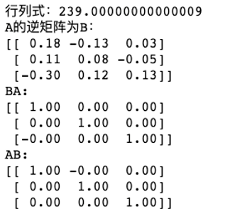
import numpy as np
# 格式化numpy输出
np.set_printoptions(formatter={'float':'{:0.2f}'.format})
A = np.array([[4,5,1],[0,8,3],[9,4,7]])

# 求行列式
print("行列式:" + str(np.linalg.det(A)))
B = np.linalg.inv(A) # 求逆
print("A的逆矩阵为B:")
print(A_inv)
print("BA:") # 结果验证
print(B.dot(A))
print("AB:")
print(A.dot(B))
什么是回归

在回归模型中,需要预测的变量叫做因变量,用来解释因变量变化的变量叫做自变量。
一元线性回归
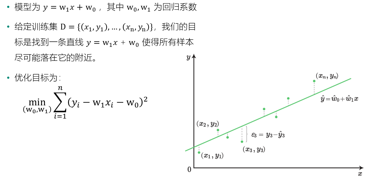
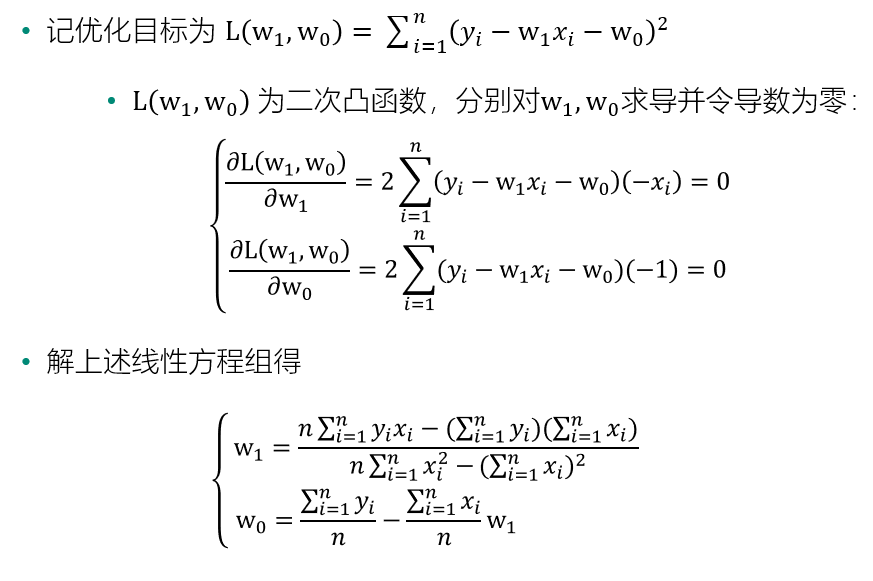
一元线性回归的求解
多线性回归

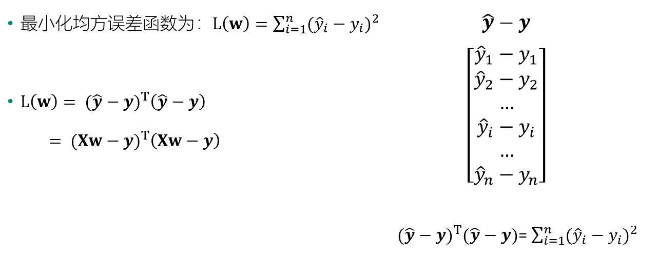
多元线性回归的矩阵表示

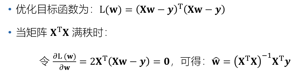
优化目标的矩阵表示
模型求解:参数估计
线性回归的问题:
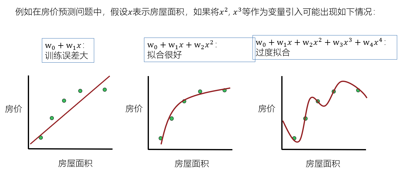
1. 实际数据可能不是线性的?
解决方法:多项式回归:使用原始特征的二次项、三次项
- 线性回归解决非线性问题
- 问题:维度灾难、过度拟合
2. 多重共线性

3. 过度拟合问题:当模型的变量过多时,线性回归可能会出现过度拟合问题
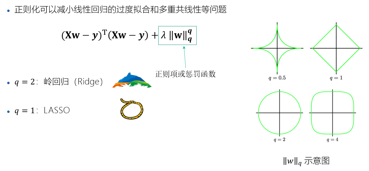
正则化
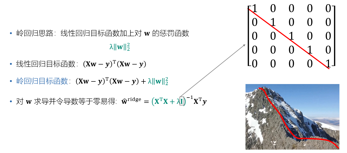
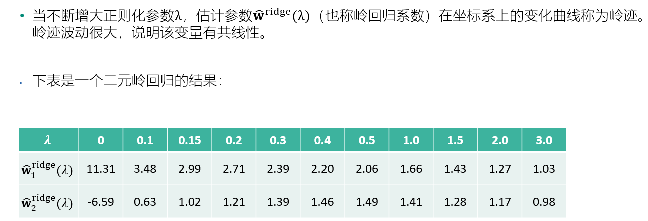
岭回归
岭迹分析
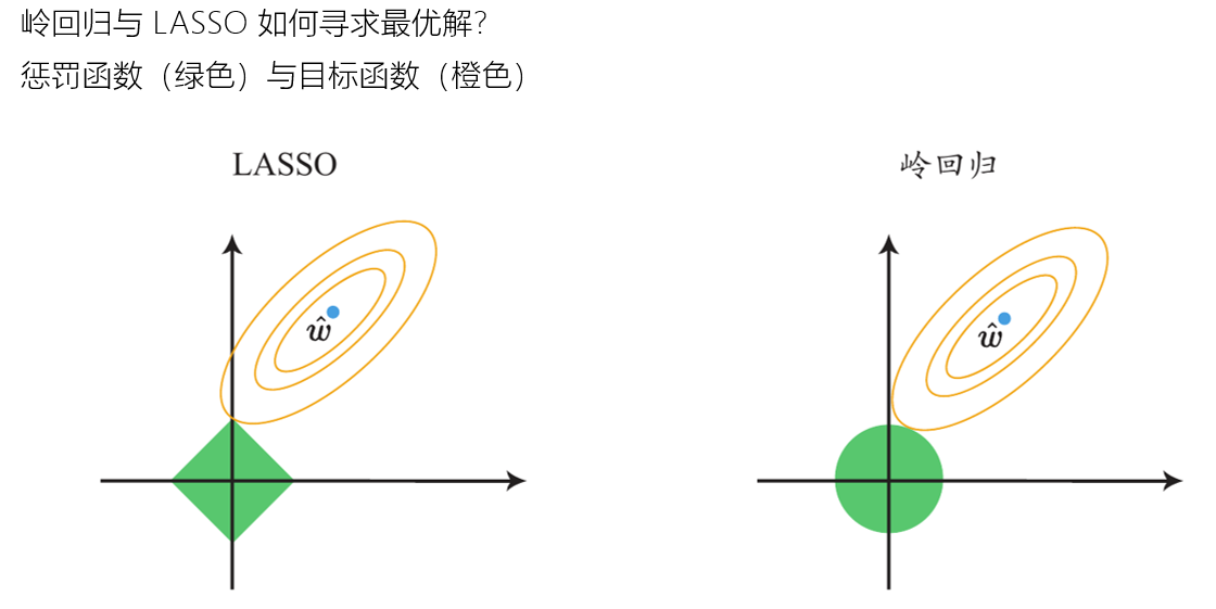
岭回归与LASSO回归
正则化路径分析

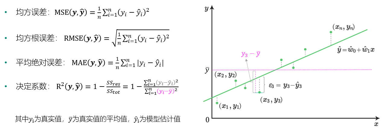
回归模型的评价指标
案例:实用回归模型预测鲍鱼年龄
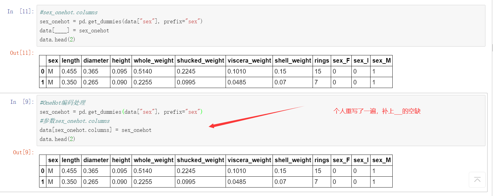
因为案例直接保存在“我的案例”中,里面已经有了相关代码,但有些地方设置成了“___”,需要自行填充,因此我会附上填充后的源码与运行截图,大部分代码和示例代码是相同的:
先发个图说明一下情况,下面是的代码是我新开了一个代码块再写了一遍:
接下来进入正题

#首先将数据集引入
import pandas as pd
import warnings
warnings.filterwarnings('ignore')
data = pd.read_csv("./input/abalone_dataset.csv")
#输出前五行
data.head()

#查看数据集中样本数量和特征数量
data.shape

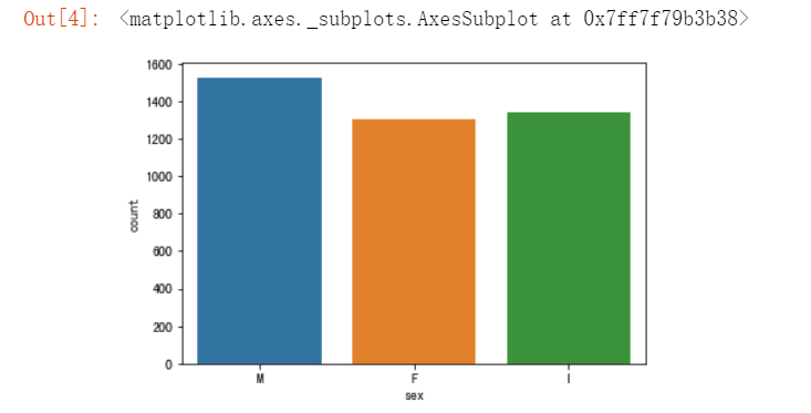
#使用seaborn绘制sex的取值分布条形图
import seaborn as sns
import matplotlib.pyplot as plt
%matplotlib inline
sns.countplot(x = "sex", data = data)
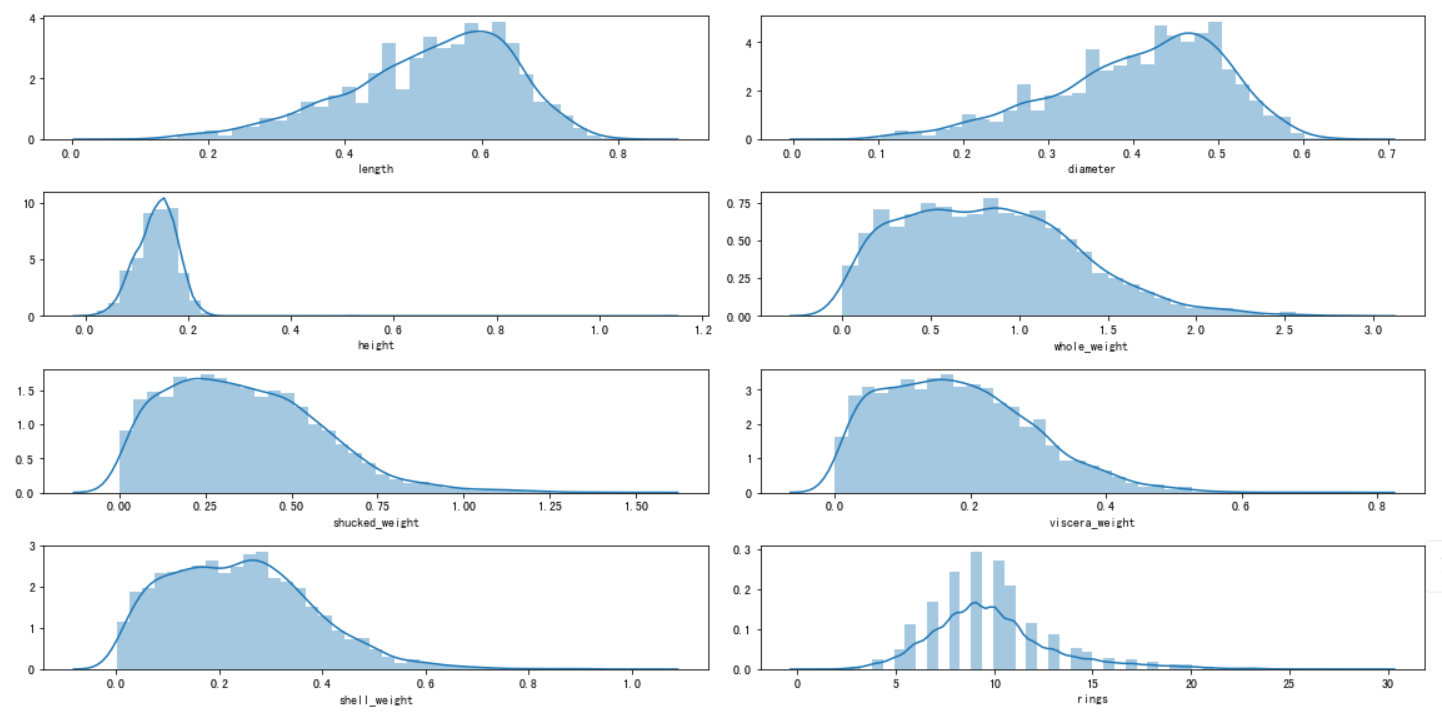
#绘制直方图观察特征取值
i = 1 # 子图记数
plt.figure(figsize=(16, 8))
for col in data.columns[1:]:
    plt.subplot(4,2,i)
    i = i + 1
    sns.distplot(data[col])
plt.tight_layout()
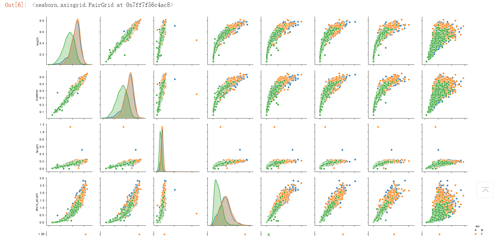
#根据sex画出不同特征之间的点缀图,seaborn提供了pairplot方法
sns.pairplot(data,hue="sex")

#计算特征之间的相关性
corr_df = data.corr()
corr_df

#为了能够直观看出关系,可以绘制热力图
fig, ax = plt.subplots(figsize=(12, 12))
#原图是绿色的,这里改成蓝色
ax = sns.heatmap(corr_df,linewidths=.5,cmap="Blues",annot=True,xticklabels=corr_df.columns, yticklabels=corr_df.index)
ax.xaxis.set_label_position('top')
ax.xaxis.tick_top()

#OneHot编码处理
sex_onehot = pd.get_dummies(data["sex"], prefix="sex")
#参数sex_onehot.columns
data[sex_onehot.columns] = sex_onehot
data.head(2)

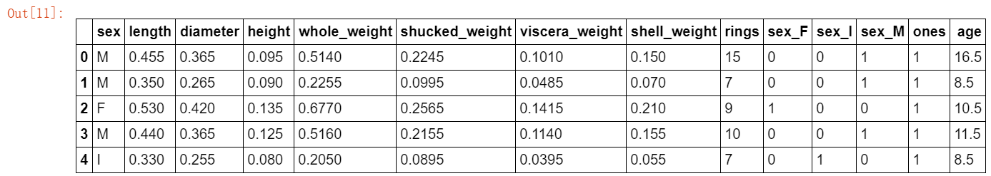
#添加取值为1的特征列
data["ones"] = 1
data.head(5)

一般每过一年,鲍鱼就会在其壳上留下一道深深的印记,这叫生长纹,就相当于树木的年轮。在本数据集中,我们要预测的是鲍鱼的年龄,可以通过环数 rings 加上 1.5 得到。所以:
#令age=rings+1.5
data["age"] = data["rings"] + 1.5
data.head(5)
将预测目标设置为 age 列,然后构造两组特征,一组包含 ones,一组不包含 ones 。对于 sex 相关的列,我们只使用 sex_F 和 sex_M。后面的模型比对中是否使用数据集的ones列会出现分歧,因此要提前分好。
#构造特征集
y = data["age"]
features_with_ones = ["length","diameter","height","whole_weight","shucked_weight","viscera_weight","shell_weight","sex_F","sex_M","ones"]
features_without_ones=["length","diameter","height","whole_weight","shucked_weight","viscera_weight","shell_weight","sex_F","sex_M"]
X = data[features_with_ones]

#训练集与测试集切分train_test_split
from sklearn import model_selection
X_train,X_test,y_train,y_test = model_selection.train_test_split(X,y,test_size=0.2, random_state=111)
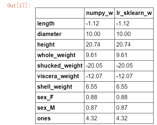
首先是线性回归:
公式及参数说明如下:

#根据公式补充参数
import numpy as np
def linear_regression(X,y):
w = np.zeros_like(X.shape[1])
if np.linalg.det(X.T.dot(X)) != 0 :
w = np.linalg.inv(X.T.dot(X)).dot(X.T).dot(y)
return w
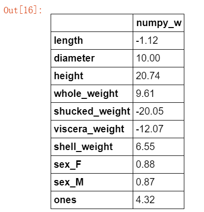
#根据模型获取系数
w1 = linear_regression(X_train,y_train)
w1 = pd.DataFrame(data = w1,index = X.columns,columns = ["numpy_w"])
w1.round(decimals=2)
这里偷个懒,直接附上案例中的说明,sklearn后面要用到多次:
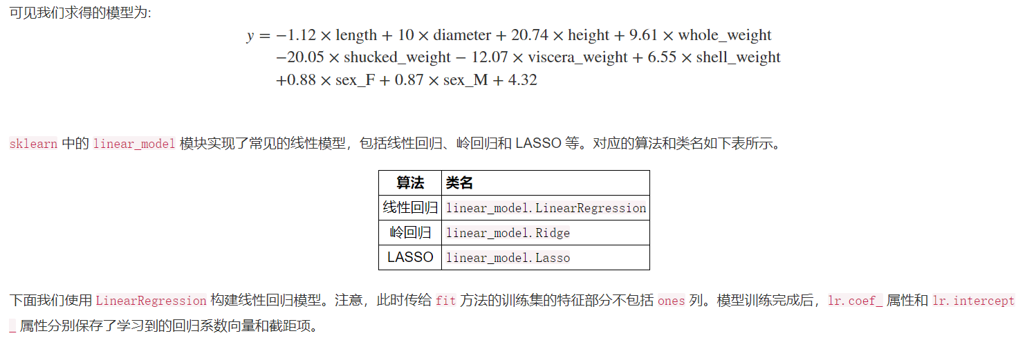
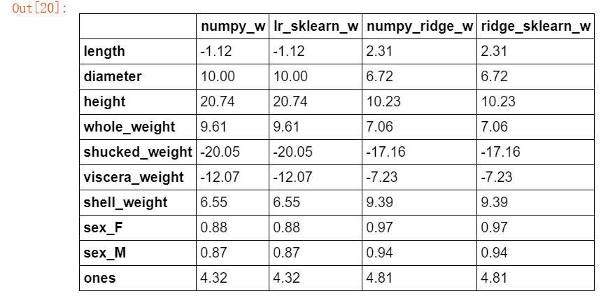
#使用之前介绍的sklearn作系数比对
from sklearn import linear_model
lr = linear_model.LinearRegression()
#刚才处理的时候将新设置的ones放了进去,而这里使用时不能添加ones列
lr.fit(X_train[features_without_ones],y_train)
w_lr = []
w_lr.extend(lr.coef_)
w_lr.append(lr.intercept_)
w1["lr_sklearn_w"] = w_lr
w1.round(decimals=2)
对比效果是一致的,证明模型构建成功。
岭回归:
公式及参数说明:

def ridge_regression(X,y,ridge_lambda):
#eye方法:生成单位矩阵
penality_matrix = np.eye(X.shape[1])
#令单位矩阵的最后一个元素=0
penality_matrix[X.shape[1] - 1][X.shape[1] - 1] = 0
#输入参数
w = np.linalg.inv(X.T.dot(X) + ridge_lambda*penality_matrix).dot(X.T).dot(y)
return w
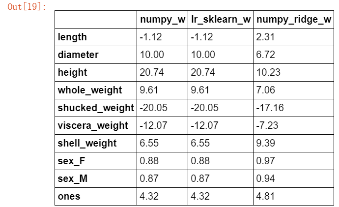
#使用岭回归模型,与之前两个模型进行比对
w2 = ridge_regression(X_train,y_train,1.0)
w1["numpy_ridge_w"] = w2
w1.round(decimals=2)
#再与sklearn中的岭回归进行对比
from sklearn.linear_model import Ridge
ridge = linear_model.Ridge(alpha=1.0)
#这里还是使用无ones列的数据集
ridge.fit(X_train[features_without_ones],y_train)
w_ridge = []
w_ridge.extend(ridge.coef_)
w_ridge.append(ridge.intercept_)
w1["ridge_sklearn_w"] = w_ridge
w1.round(decimals=2)
LASSO:
LASSO的解没有公式(上面已经提到过),因此直接使用函数构建:
#使用LASSO
from sklearn.linear_model import Lasso
#alpha设置要小一些,否则
lasso = linear_model.Lasso(alpha=1)
lasso.fit(X_train[features_without_ones],y_train)
print(lasso.coef_)
print(lasso.intercept_)
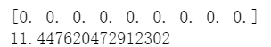
上边示范一下当alpha参数设置过大时的情况
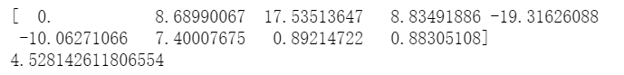
因此设置适当的值:
from sklearn.linear_model import Lasso
#因此设置0.001,设置值越小压缩越小,因为这次案例使用的数据集容量本就不多
lasso = linear_model.Lasso(alpha=0.001)
lasso.fit(X_train[features_without_ones],y_train)
print(lasso.coef_)
print(lasso.intercept_)
模型评估:
MAE:
#平均绝对误差MAE
##使用sklearn.metrics进行预测
from sklearn.metrics import mean_absolute_error
#线性回归
y_test_pred_lr = lr.predict(X_test.iloc[:,:-1])
print(round(mean_absolute_error(y_test,y_test_pred_lr),4))

#岭回归
y_test_pred_ridge = ridge.predict(X_test[features_without_ones])
print(round(mean_absolute_error(y_test,y_test_pred_ridge),4))

#LASSO
y_test_pred_lasso = lasso.predict(X_test[features_without_ones])
print(round(mean_absolute_error(y_test,y_test_pred_lasso),4))

R2:
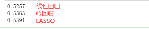
#决定系数R2
from sklearn.metrics import r2_score
#线性回归
print(round(r2_score(y_test,y_test_pred_lr),4))
#岭回归
print(round(r2_score(y_test,y_test_pred_ridge),4))
#LASSO
print(round(r2_score(y_test,y_test_pred_lasso),4))
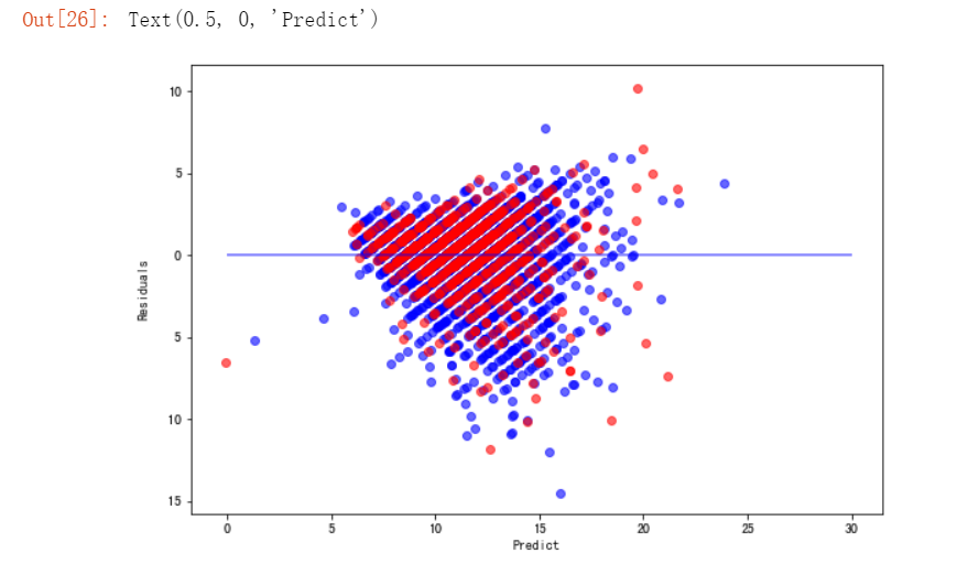
残差图:
#构建残差图进行诊断
##横轴是模型的预测值,纵轴是预测值与真实值的差距
plt.figure(figsize=(9, 6))
y_train_pred_ridge = ridge.predict(X_train[features_without_ones])
plt.scatter(y_train_pred_ridge, y_train_pred_ridge - y_train, c="b", alpha=0.6)
plt.scatter(y_test_pred_ridge, y_test_pred_ridge - y_test, c="r",alpha=0.6)
plt.hlines(y=0, xmin=0, xmax=30,color="b",alpha=0.6)
plt.ylabel("Residuals")
plt.xlabel("Predict")
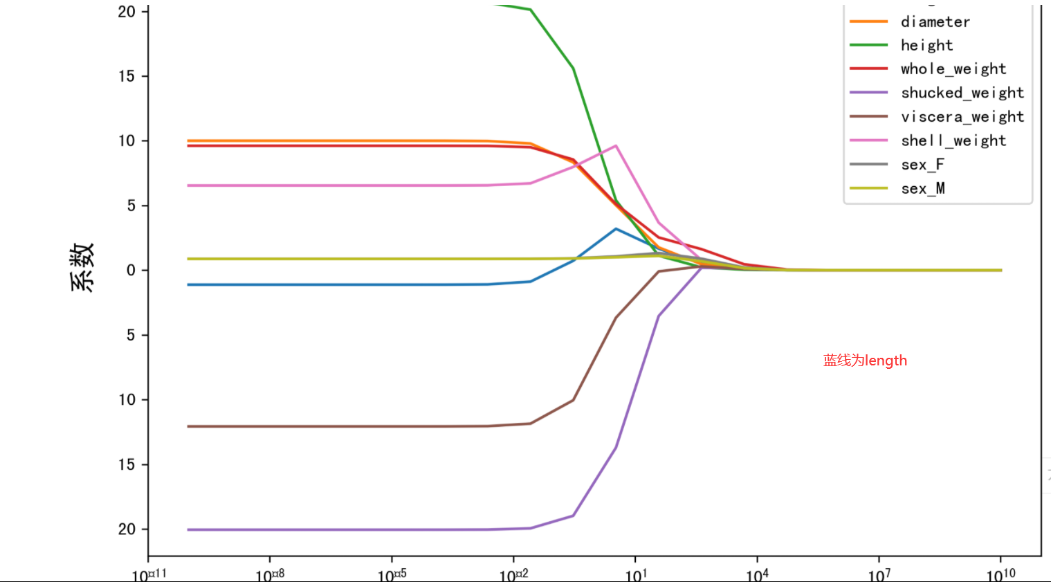
岭迹:
#构建岭迹
alphas = np.logspace(-10,10,20)
coef = pd.DataFrame()
for alpha in alphas:
    ridge_clf = Ridge(alpha=alpha)
    ridge_clf.fit(X_train[features_without_ones],y_train)
    df = pd.DataFrame([ridge_clf.coef_],columns=X_train[features_without_ones].columns)
    df['alpha'] = alpha
    coef = coef.append(df,ignore_index=True)
coef.head().round(decimals=2)

#根据刚才构建好的数据,进行绘图
plt.rcParams['figure.dpi'] = 300 #分辨率
plt.figure(figsize=(9, 6))
coef['alpha'] = coef['alpha']

for feature in X_train.columns[:-1]:
    plt.plot('alpha',feature,data=coef)
ax = plt.gca()
ax.set_xscale('log')
plt.legend(loc='upper right')
plt.xlabel(r'$alpha$',fontsize=15)
plt.ylabel('系数',fontsize=15)

plt.show()
LASSO的正则化路径:
#绘制LASSO的正则化路径
##数据准备
coef = pd.DataFrame()
for alpha in np.linspace(0.0001,0.2,20):
    lasso_clf = Lasso(alpha=alpha)
    lasso_clf.fit(X_train[features_without_ones],y_train)
    df = pd.DataFrame([lasso_clf.coef_],columns=X_train[features_without_ones].columns)
    df['alpha'] = alpha
    coef = coef.append(df,ignore_index=True)
coef.head()
##绘图
plt.figure(figsize=(9, 6))
for feature in X_train.columns[:-1]:
    plt.plot('alpha',feature,data=coef)
plt.legend(loc='upper right')
plt.xlabel(r'$alpha$',fontsize=15)
plt.ylabel('系数',fontsize=15)
plt.show()

总结:
