一、线性回归
1、简单线性回归
a、
> x = women
> x
   height weight
1      58    115
2      59    117
3      60    120
4      61    123
5      62    126
6      63    129
7      64    132
8      65    135
9      66    139
10     67    142
11     68    146
12     69    150
13     70    154
14     71    159
15     72    164
> fit = lm(weight ~ height, data=x)
> summary(fit)

Call:
lm(formula = weight ~ height, data = x)

Residuals:
    Min      1Q  Median      3Q     Max
-1.7333 -1.1333 -0.3833  0.7417  3.1167

Coefficients:
             Estimate Std. Error t value Pr(>|t|)
(Intercept) -87.51667    5.93694  -14.74 1.71e-09 ***
height        3.45000    0.09114   37.85 1.09e-14 ***
---
Signif. codes:  0 ‘***’ 0.001 ‘**’ 0.01 ‘*’ 0.05 ‘.’ 0.1 ‘ ’ 1

Residual standard error: 1.525 on 13 degrees of freedom
Multiple R-squared:  0.991,    Adjusted R-squared:  0.9903
F-statistic:  1433 on 1 and 13 DF,  p-value: 1.091e-14

> fitted(fit)
       1        2        3        4        5        6        7        8        9
112.5833 116.0333 119.4833 122.9333 126.3833 129.8333 133.2833 136.7333 140.1833
      10       11       12       13       14       15
143.6333 147.0833 150.5333 153.9833 157.4333 160.8833
> women$weight
 [1] 115 117 120 123 126 129 132 135 139 142 146 150 154 159 164
> residuals(fit)
          1           2           3           4           5           6           7
 2.41666667  0.96666667  0.51666667  0.06666667 -0.38333333 -0.83333333 -1.28333333
          8           9          10          11          12          13          14
-1.73333333 -1.18333333 -1.63333333 -1.08333333 -0.53333333  0.01666667  1.56666667
         15
 3.11666667
> plot(women$height, women$weight)
> abline(fit)

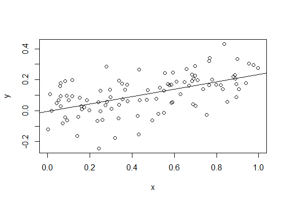
b、
> x = runif(100)
> y = 0.2*x + 0.1*rnorm(100)
> fit = lm(y~x)
> summary(fit)

Call:
lm(formula = y ~ x)

Residuals:
      Min        1Q    Median        3Q       Max
-0.299493 -0.056850  0.004709  0.066714  0.237272

Coefficients:
             Estimate Std. Error t value Pr(>|t|)
(Intercept) -0.002891   0.019688  -0.147    0.884
x            0.236938   0.036158   6.553 2.64e-09 ***
---
Signif. codes:  0 ‘***’ 0.001 ‘**’ 0.01 ‘*’ 0.05 ‘.’ 0.1 ‘ ’ 1

Residual standard error: 0.1037 on 98 degrees of freedom
Multiple R-squared:  0.3047,    Adjusted R-squared:  0.2976
F-statistic: 42.94 on 1 and 98 DF,  p-value: 2.639e-09

> plot(x,y)
> abline(fit)
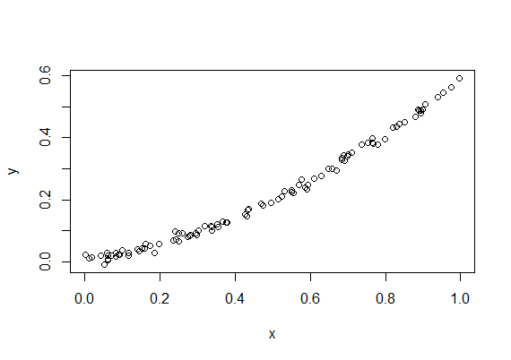
c、
> y = 0.2*x + 0.01*rnorm(100)
> fit = lm(y~x)
> summary(fit)

Call:
lm(formula = y ~ x)

Residuals:
      Min        1Q    Median        3Q       Max
-0.019936 -0.005549 -0.001135  0.004598  0.026435

Coefficients:
             Estimate Std. Error t value Pr(>|t|)
(Intercept) -0.002684   0.001837  -1.461    0.147
x            0.203561   0.003374  60.326   <2e-16 ***
---
Signif. codes:  0 ‘***’ 0.001 ‘**’ 0.01 ‘*’ 0.05 ‘.’ 0.1 ‘ ’ 1

Residual standard error: 0.009678 on 98 degrees of freedom
Multiple R-squared:  0.9738,    Adjusted R-squared:  0.9735
F-statistic:  3639 on 1 and 98 DF,  p-value: < 2.2e-16

> plot(x,y)
> abline(fit)

2、多项式线性回归
a、
> fit2 = lm(weight ~ height + I(height^2), data=women)
> summary(fit2)

Call:
lm(formula = weight ~ height + I(height^2), data = women)

Residuals:
     Min       1Q   Median       3Q      Max
-0.50941 -0.29611 -0.00941  0.28615  0.59706

Coefficients:
             Estimate Std. Error t value Pr(>|t|)
(Intercept) 261.87818   25.19677  10.393 2.36e-07 ***
height       -7.34832    0.77769  -9.449 6.58e-07 ***
I(height^2)   0.08306    0.00598  13.891 9.32e-09 ***
---
Signif. codes:  0 ‘***’ 0.001 ‘**’ 0.01 ‘*’ 0.05 ‘.’ 0.1 ‘ ’ 1

Residual standard error: 0.3841 on 12 degrees of freedom
Multiple R-squared:  0.9995,    Adjusted R-squared:  0.9994
F-statistic: 1.139e+04 on 2 and 12 DF,  p-value: < 2.2e-16

> plot(women$height, women$weight)
> lines(women$height, fitted(fit2))

b、
> y = 0.4*x**2 + 0.2*x + 0.01*rnorm(100)
> fit = lm(y~x + I(x^2))
> summary(fit)

Call:
lm(formula = y ~ x + I(x^2))

Residuals:
       Min         1Q     Median         3Q        Max
-0.0243909 -0.0058432 -0.0000949  0.0056788  0.0245737

Coefficients:
            Estimate Std. Error t value Pr(>|t|)
(Intercept) 0.003611   0.002727   1.324    0.189
x           0.189098   0.013571  13.934   <2e-16 ***
I(x^2)      0.400631   0.013806  29.018   <2e-16 ***
---
Signif. codes:  0 ‘***’ 0.001 ‘**’ 0.01 ‘*’ 0.05 ‘.’ 0.1 ‘ ’ 1

Residual standard error: 0.009857 on 97 degrees of freedom
Multiple R-squared:  0.9966,    Adjusted R-squared:  0.9965
F-statistic: 1.418e+04 on 2 and 97 DF,  p-value: < 2.2e-16

> plot(x,y)
3、多元线性回归
> states = as.data.frame(state.x77[, c("Murder", "Population", "Illiteracy", "Income", "Frost")])
> cor(states)
               Murder Population Illiteracy     Income      Frost
Murder      1.0000000  0.3436428  0.7029752 -0.2300776 -0.5388834
Population  0.3436428  1.0000000  0.1076224  0.2082276 -0.3321525
Illiteracy  0.7029752  0.1076224  1.0000000 -0.4370752 -0.6719470
Income     -0.2300776  0.2082276 -0.4370752  1.0000000  0.2262822
Frost      -0.5388834 -0.3321525 -0.6719470  0.2262822  1.0000000

> install.packages("car")
> library(car)
> scatterplotMatrix(states, spread=FALSE, lty.smooth=2, main="Scatter Plot Matrix")

> fit = lm(Murder ~ Population + Illiteracy + Income + Frost, data=states)
> summary(fit)

Call:
lm(formula = Murder ~ Population + Illiteracy + Income + Frost,
    data = states)

Residuals:
    Min      1Q  Median      3Q     Max
-4.7960 -1.6495 -0.0811  1.4815  7.6210

Coefficients:
             Estimate Std. Error t value Pr(>|t|)
(Intercept) 1.235e+00  3.866e+00   0.319   0.7510
Population  2.237e-04  9.052e-05   2.471   0.0173 *
Illiteracy  4.143e+00  8.744e-01   4.738 2.19e-05 ***
Income      6.442e-05  6.837e-04   0.094   0.9253
Frost       5.813e-04  1.005e-02   0.058   0.9541
---
Signif. codes:  0 ‘***’ 0.001 ‘**’ 0.01 ‘*’ 0.05 ‘.’ 0.1 ‘ ’ 1

Residual standard error: 2.535 on 45 degrees of freedom
Multiple R-squared:  0.567,    Adjusted R-squared:  0.5285
F-statistic: 14.73 on 4 and 45 DF,  p-value: 9.133e-08
4、有叫互项的多元线性回归
> fit = lm(mpg ~ hp + wt + hp:wt, data=mtcars)
> summary(fit)

Call:
lm(formula = mpg ~ hp + wt + hp:wt, data = mtcars)

Residuals:
    Min      1Q  Median      3Q     Max
-3.0632 -1.6491 -0.7362  1.4211  4.5513

Coefficients:
            Estimate Std. Error t value Pr(>|t|)
(Intercept) 49.80842    3.60516  13.816 5.01e-14 ***
hp          -0.12010    0.02470  -4.863 4.04e-05 ***
wt          -8.21662    1.26971  -6.471 5.20e-07 ***
hp:wt        0.02785    0.00742   3.753 0.000811 ***
---
Signif. codes:  0 ‘***’ 0.001 ‘**’ 0.01 ‘*’ 0.05 ‘.’ 0.1 ‘ ’ 1

Residual standard error: 2.153 on 28 degrees of freedom
Multiple R-squared:  0.8848,    Adjusted R-squared:  0.8724
F-statistic: 71.66 on 3 and 28 DF,  p-value: 2.981e-13
马力与车重的叫互项是显著的,说明:响应变量与其中一个预测变量的关系依赖于另外一个预测变量的水平。
> install.packages("effects")
> library(effects)
> plot(effect("hp:wt", fit, list(wt=c(2.2, 3.2, 4.2))), multiline=TRUE)
