PCA python 实现

PCA 实现：

参考博客：https://blog.csdn.net/u013719780/article/details/78352262

from __future__ import print_function
from sklearn import datasets
import matplotlib.pyplot as plt
import matplotlib.cm as cmx
import matplotlib.colors as colors
import numpy as np
# matplotlib inline



def shuffle_data(X, y, seed=None):
    if seed:
        np.random.seed(seed)

    idx = np.arange(X.shape[0])
    np.random.shuffle(idx)

    return X[idx], y[idx]



# 正规化数据集 X
def normalize(X, axis=-1, p=2):
    lp_norm = np.atleast_1d(np.linalg.norm(X, p, axis))
    lp_norm[lp_norm == 0] = 1
    return X / np.expand_dims(lp_norm, axis)


# 标准化数据集 X
def standardize(X):
    X_std = np.zeros(X.shape)
    mean = X.mean(axis=0)
    std = X.std(axis=0)

    # 做除法运算时请永远记住分母不能等于0的情形
    # X_std = (X - X.mean(axis=0)) / X.std(axis=0) 
    for col in range(np.shape(X)[1]):
        if std[col]:
            X_std[:, col] = (X_std[:, col] - mean[col]) / std[col]

    return X_std


# 划分数据集为训练集和测试集
def train_test_split(X, y, test_size=0.2, shuffle=True, seed=None):
    if shuffle:
        X, y = shuffle_data(X, y, seed)

    n_train_samples = int(X.shape[0] * (1-test_size))
    x_train, x_test = X[:n_train_samples], X[n_train_samples:]
    y_train, y_test = y[:n_train_samples], y[n_train_samples:]

    return x_train, x_test, y_train, y_test



# 计算矩阵X的协方差矩阵
def calculate_covariance_matrix(X, Y=np.empty((0,0))):
    if not Y.any():
        Y = X
    n_samples = np.shape(X)[0]
    covariance_matrix = (1 / (n_samples-1)) * (X - X.mean(axis=0)).T.dot(Y - Y.mean(axis=0))

    return np.array(covariance_matrix, dtype=float)


# 计算数据集X每列的方差
def calculate_variance(X):
    n_samples = np.shape(X)[0]
    variance = (1 / n_samples) * np.diag((X - X.mean(axis=0)).T.dot(X - X.mean(axis=0)))
    return variance


# 计算数据集X每列的标准差
def calculate_std_dev(X):
    std_dev = np.sqrt(calculate_variance(X))
    return std_dev


# 计算相关系数矩阵
def calculate_correlation_matrix(X, Y=np.empty([0])):
    # 先计算协方差矩阵
    covariance_matrix = calculate_covariance_matrix(X, Y)
    # 计算X, Y的标准差
    std_dev_X = np.expand_dims(calculate_std_dev(X), 1)
    std_dev_y = np.expand_dims(calculate_std_dev(Y), 1)
    correlation_matrix = np.divide(covariance_matrix, std_dev_X.dot(std_dev_y.T))

    return np.array(correlation_matrix, dtype=float)



class PCA():
    """
    主成份分析算法PCA，非监督学习算法.
    """
    def __init__(self):
        self.eigen_values = None
        self.eigen_vectors = None
        self.k = 2

    def transform(self, X):
        """ 
        将原始数据集X通过PCA进行降维
        """
        covariance = calculate_covariance_matrix(X)

        # 求解特征值和特征向量
        self.eigen_values, self.eigen_vectors = np.linalg.eig(covariance)

        # 将特征值从大到小进行排序，注意特征向量是按列排的，即self.eigen_vectors第k列是self.eigen_values中第k个特征值对应的特征向量
        idx = self.eigen_values.argsort()[::-1]
        eigenvalues = self.eigen_values[idx][:self.k]
        eigenvectors = self.eigen_vectors[:, idx][:, :self.k]

        # 将原始数据集X映射到低维空间
        X_transformed = X.dot(eigenvectors)

        return X_transformed


def main():
    # Load the dataset
    data = datasets.load_iris()
    X = data.data
    y = data.target

    # 将数据集X映射到低维空间
    X_trans = PCA().transform(X)

    x1 = X_trans[:, 0]
    x2 = X_trans[:, 1]

    print(X[0:2])

    cmap = plt.get_cmap('viridis')
    colors = [cmap(i) for i in np.linspace(0, 1, len(np.unique(y)))]

    class_distr = []
    # Plot the different class distributions
    for i, l in enumerate(np.unique(y)):
        _x1 = x1[y == l]
        _x2 = x2[y == l]
        _y = y[y == l]
        class_distr.append(plt.scatter(_x1, _x2, color=colors[i]))

    # Add a legend
    plt.legend(class_distr, y, loc=1)

    # Axis labels
    plt.xlabel('Principal Component 1')
    plt.ylabel('Principal Component 2')
    plt.show()


if __name__ == "__main__":
    main()

　　

kPCA

1、核主成份分析 Kernel Principle Component Analysis:

1）现实世界中，并不是所有数据都是线性可分的
2）通过LDA，PCA将其转化为线性问题并不是好的方法

3）线性可分 VS 非线性可分

2、引入核主成份分析：

可以通过kPCA将非线性数据映射到高维空间，在高维空间下使用标准PCA将其映射到另一个低维空间

3、原理:
定义非线性映射函数，该函数可以对原始特征进行非线性组合，以将原始的d维数据集映射到更高维的k维特征空间。

1)多项式核
2)双曲正切核
3)径向基核（RBF），高斯核函数

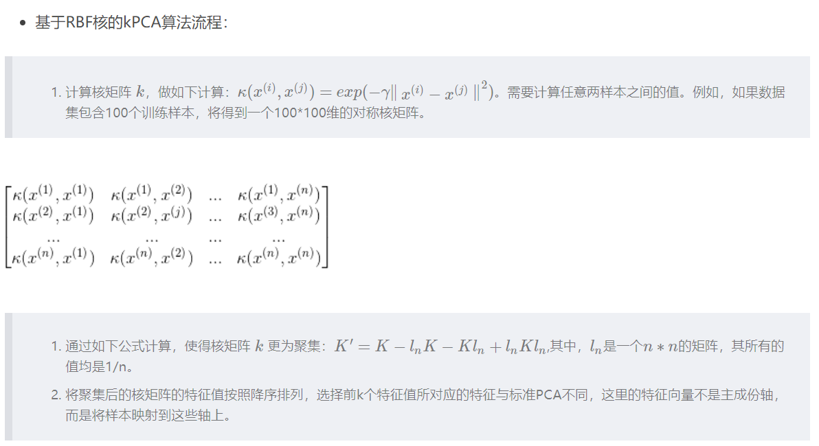
基于RBF核的kPCA算法流程：

Python 代码：

from scipy.spatial.distance import pdist, squareform
from scipy import exp
from numpy.linalg import eigh
import numpy as np

def rbf_kernel_pca(X, gamma, n_components):
    """
    RBF kernel PCA implementation.

    Parameters
    ------------
    X: {NumPy ndarray}, shape = [n_samples, n_features]

    gamma: float
      Tuning parameter of the RBF kernel

    n_components: int
      Number of principal components to return

    Returns
    ------------
     X_pc: {NumPy ndarray}, shape = [n_samples, k_features]
       Projected dataset   

    """
    # Calculate pairwise squared Euclidean distances
    # in the MxN dimensional dataset.
    sq_dists = pdist(X, 'sqeuclidean')

    # Convert pairwise distances into a square matrix.
    mat_sq_dists = squareform(sq_dists)

    # Compute the symmetric kernel matrix.
    K = exp(-gamma * mat_sq_dists)

    # Center the kernel matrix.
    N = K.shape[0]
    one_n = np.ones((N, N)) / N
    K = K - one_n.dot(K) - K.dot(one_n) + one_n.dot(K).dot(one_n)

    # Obtaining eigenpairs from the centered kernel matrix
    # numpy.linalg.eigh returns them in sorted order
    eigvals, eigvecs = eigh(K)

    # Collect the top k eigenvectors (projected samples)
    X_pc = np.column_stack((eigvecs[:, -i]
                            for i in range(1, n_components + 1)))

    return X_pc






import matplotlib.pyplot as plt
from sklearn.datasets import make_moons

X, y = make_moons(n_samples=100, random_state=123)

plt.scatter(X[y == 0, 0], X[y == 0, 1], color='red', marker='^', alpha=0.5)
plt.scatter(X[y == 1, 0], X[y == 1, 1], color='blue', marker='o', alpha=0.5)

plt.tight_layout()
# plt.savefig('./figures/half_moon_1.png', dpi=300)
plt.show()


# 直接用PCA
from sklearn.decomposition import PCA
from sklearn.preprocessing import StandardScaler

scikit_pca = PCA(n_components=2)
X_spca = scikit_pca.fit_transform(X)

fig, ax = plt.subplots(nrows=1, ncols=2, figsize=(7, 3))

ax[0].scatter(X_spca[y == 0, 0], X_spca[y == 0, 1],
              color='red', marker='^', alpha=0.5)
ax[0].scatter(X_spca[y == 1, 0], X_spca[y == 1, 1],
              color='blue', marker='o', alpha=0.5)

ax[1].scatter(X_spca[y == 0, 0], np.zeros((50, 1)) + 0.02,
              color='red', marker='^', alpha=0.5)
ax[1].scatter(X_spca[y == 1, 0], np.zeros((50, 1)) - 0.02,
              color='blue', marker='o', alpha=0.5)

ax[0].set_xlabel('PC1')
ax[0].set_ylabel('PC2')
ax[1].set_ylim([-1, 1])
ax[1].set_yticks([])
ax[1].set_xlabel('PC1')

plt.tight_layout()
# plt.savefig('./figures/half_moon_2.png', dpi=300)
plt.show()


＃　KPCA

from matplotlib.ticker import FormatStrFormatter

X_kpca = rbf_kernel_pca(X, gamma=15, n_components=2)

fig, ax = plt.subplots(nrows=1,ncols=2, figsize=(7,3))
ax[0].scatter(X_kpca[y==0, 0], X_kpca[y==0, 1], 
            color='red', marker='^', alpha=0.5)
ax[0].scatter(X_kpca[y==1, 0], X_kpca[y==1, 1],
            color='blue', marker='o', alpha=0.5)

ax[1].scatter(X_kpca[y==0, 0], np.zeros((50,1))+0.02, 
            color='red', marker='^', alpha=0.5)
ax[1].scatter(X_kpca[y==1, 0], np.zeros((50,1))-0.02,
            color='blue', marker='o', alpha=0.5)

ax[0].set_xlabel('PC1')
ax[0].set_ylabel('PC2')
ax[1].set_ylim([-1, 1])
ax[1].set_yticks([])
ax[1].set_xlabel('PC1')
ax[0].xaxis.set_major_formatter(FormatStrFormatter('%0.1f'))
ax[1].xaxis.set_major_formatter(FormatStrFormatter('%0.1f'))

plt.tight_layout()
# plt.savefig('./figures/half_moon_3.png', dpi=300)
plt.show()



＃sklearn kpca

from sklearn.decomposition import KernelPCA

X, y = make_moons(n_samples=100, random_state=123)
scikit_kpca = KernelPCA(n_components=2, kernel='rbf', gamma=15)
X_skernpca = scikit_kpca.fit_transform(X)

plt.scatter(X_skernpca[y == 0, 0], X_skernpca[y == 0, 1],
            color='red', marker='^', alpha=0.5)
plt.scatter(X_skernpca[y == 1, 0], X_skernpca[y == 1, 1],
            color='blue', marker='o', alpha=0.5)

plt.xlabel('PC1')
plt.ylabel('PC2')
plt.tight_layout()
# plt.savefig('./figures/scikit_kpca.png', dpi=300)
plt.show()

　　

参考： https://blog.csdn.net/weixin_40604987/article/details/79632888