浅谈压缩感知（二十九）：压缩感知算法之迭代硬阈值（IHT）

主要内容：

1、IHT的算法流程

2、IHT的MATLAB实现

3、二维信号的实验与结果

4、加速的IHT算法实验与结果

一、IHT的算法流程

文献：T. Blumensath and M. Davies, "Iterative Hard Thresholding for Compressed Sensing," 2008.

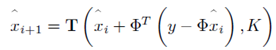
基本思想：给定一个初始的X0，然后通过以下的阈值公式不断地迭代。

二、IHT的MATLAB实现

function hat_x=cs_iht(y,T_Mat,s_ratio,m)
% y=T_Mat*x, T_Mat is n-by-m
% y - measurements
% T_Mat - combination of random matrix and sparse representation basis
% s_ratio - sparsity percentage of original signal
% m - size of the original signal
% the sparsity is length(y)/4

hat_x_tp=zeros(m,1);         % initialization with the size of original 
s=floor(length(y)*s_ratio);        % sparsity
u=0.5;                       % impact factor

% T_Mat=T_Mat/sqrt(sum(sum(T_Mat.^2))); % normalizae the whole matrix

for times=1:s
    
    x_increase=T_Mat'*(y-T_Mat*hat_x_tp);
    
    hat_x=hat_x_tp+u*x_increase;
    
    [val,pos]=sort(abs(hat_x),'descend');  
    
    hat_x(pos(s+1:end))=0;   % thresholding, keeping the larges s elements

    hat_x_tp=hat_x;          % update

end

三、二维信号的实验与结果

function Demo_CS_IHT()
%%%%%%%%%%%%%%%%%%%%%%%%%%%%%%%%%%%%%%%%%%%%%%%%%%%%%%%%%%%%%%%%%%%%%%%%%%%
% the DCT basis is selected as the sparse representation dictionary
% instead of seting the whole image as a vector, I process the image in the
% fashion of column-by-column, so as to reduce the complexity.

% Author: Chengfu Huo, roy@mail.ustc.edu.cn, http://home.ustc.edu.cn/~roy
% Reference: T. Blumensath and M. Davies, “Iterative Hard Thresholding for
% Compressed Sensing,” 2008.
%%%%%%%%%%%%%%%%%%%%%%%%%%%%%%%%%%%%%%%%%%%%%%%%%%%%%%%%%%%%%%%%%%%%%%%%%%%

%------------ read in the image --------------
img=imread('lena.bmp');     % testing image
img=double(img);
[height,width]=size(img);


%------------ form the measurement matrix and base matrix ---------------
Phi=randn(floor(height/3),width);  % only keep one third of the original data  
Phi = Phi./repmat(sqrt(sum(Phi.^2,1)),[floor(height/3),1]); % normalize each column

mat_dct_1d=zeros(256,256);  % building the DCT basis (corresponding to each column)
for k=0:1:255 
    dct_1d=cos([0:1:255]'*k*pi/256);
    if k>0
        dct_1d=dct_1d-mean(dct_1d); 
    end;
    mat_dct_1d(:,k+1)=dct_1d/norm(dct_1d);
end


%--------- projection ---------
img_cs_1d=Phi*img;          % treat each column as a independent signal


%-------- recover using iht ------------
sparse_rec_1d=zeros(height,width);            
Theta_1d=Phi*mat_dct_1d;
s_ratio = 0.2;
for i=1:width
    column_rec=cs_iht(img_cs_1d(:,i),Theta_1d,s_ratio,height);
    sparse_rec_1d(:,i)=column_rec';           % sparse representation
end
img_rec_1d=mat_dct_1d*sparse_rec_1d;          % inverse transform


%------------ show the results --------------------
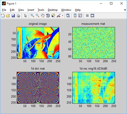
figure(1)
% subplot(2,2,1),imagesc(img),title('original image')
subplot(2,2,1),imshow(img,[]),title('original image')
subplot(2,2,2),imagesc(Phi),title('measurement mat')
subplot(2,2,3),imagesc(mat_dct_1d),title('1d dct mat')
psnr = 20*log10(255/sqrt(mean((img(:)-img_rec_1d(:)).^2)));
% subplot(2,2,4),imagesc(img_rec_1d),title(strcat('1d rec img ',num2str(psnr),'dB'))
subplot(2,2,4),imshow(img_rec_1d,[]),title(strcat('1d rec img ',num2str(psnr),'dB'))

disp('over')


%************************************************************************%
function hat_x=cs_iht(y,T_Mat,s_ratio,m)
% y=T_Mat*x, T_Mat is n-by-m
% y - measurements
% T_Mat - combination of random matrix and sparse representation basis
% s_ratio - sparsity percentage of original signal
% m - size of the original signal
% the sparsity is length(y)/4

hat_x_tp=zeros(m,1);         % initialization with the size of original 
s=floor(length(y)*s_ratio);        % sparsity
u=0.5;                       % impact factor

% T_Mat=T_Mat/sqrt(sum(sum(T_Mat.^2))); % normalizae the whole matrix

for times=1:s
    
    x_increase=T_Mat'*(y-T_Mat*hat_x_tp);
    
    hat_x=hat_x_tp+u*x_increase;
    
    [val,pos]=sort(abs(hat_x),'descend');  
    
    hat_x(pos(s+1:end))=0;   % thresholding, keeping the larges s elements

    hat_x_tp=hat_x;          % update

end

结论：实验针对的是图像信号，但算法中运用的是1维的算法，因此实验结果不太理想。（后面提供一个链接，有更好的代码 hard_l0_Mterm.m）

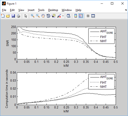
四、加速的IHT算法实验与结果

文献：Blumensath T. Accelerated iterative hard thresholding[J]. Signal Processing, 2012, 92(3): 752-756.

五、相关代码

http://www.personal.soton.ac.uk/tb1m08/sparsify/sparsify.html