引言:
Normal Equation 是最基础的最小二乘方法。在Andrew Ng的课程中给出了矩阵推到形式,本文将重点提供几种推导方式以便于全方位帮助Machine Learning用户学习。
Notations:
RSS(Residual Sum Squared error):残差平方和
β:参数列向量
X:N×p 矩阵,每行是输入的样本向量
y:标签列向量,即目标列向量
Method 1. 向量投影在特征纬度(Vector Projection onto the Column Space)
是一种最直观的理解: The optimization of linear regression is equivalent to finding the projection of vector y onto the column space of X. As the projection is denoted by Xβ, the optimal configuration of β is when the error vector y−Xβ is orthogonal to the column space of X, that is
XT(y−Xβ)=0 (1)
Solving this gives:
β=(XTX)−1XTy.
Method 2. Direct Matrix Differentiation
通过重写S(β)为简单形式是一种最简明的方法
S(β)=(y−Xβ)T(y−Xβ)=yTy−βTXTy−yTXβ+βTXTXβ=yTy−2βTXTy+βTXTXβ.
注意上式最后一步转化:Xβ是vector,所以和其他矩阵相乘的顺序无关紧要,(xβ)Ty=yT(xβ).
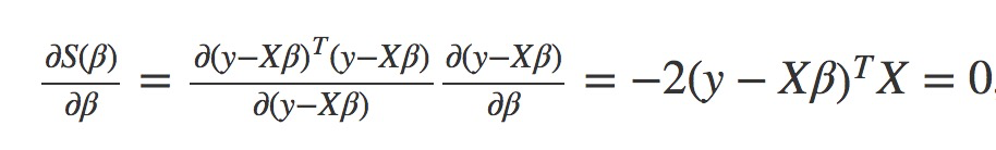
To find where the above function has a minimum, will derive by β and compare to 0.
−2yTX+βT(XTX+(XTX)T)=−2yTX+2βTXTX=0,
Solving S(β) gives:
β=(XTX)−1XTy.
Method 3. Matrix Differentiation with Chain-rule
这种方式对懒人来说最简单: it takes very little effort to reach the solution. The key is to apply the chain-rule:
solving S(β) gives:
β=(XTX)−1XTy.
This method requires an understanding of matrix differentiation of the quadratic form below: ![]()
Method 4. Without Matrix Differentiation
We can rewrite S(β) as following:
S(β)=⟨β,β⟩−2⟨β,(XTX)−1XTy⟩+⟨(XTX)−1XTy,(XTX)−1XTy⟩+C,
where ⟨⋅,⋅⟩ is the inner product defined by
⟨x,y⟩=xT(XTX)y.
The idea is to rewrite S(β) into the form of S(β)=(x−a)2+b such that x can be solved exactly.
Method 5. Statistical Learning Theory
An alternative method to derive the normal equation arises from the statistical learning theory. The aim of this task is to minimize the expected prediction error given by:
EPE(β)=∫(y−xTβ)Pr(dx,dy),
where x stands for a column vector of random variables, y denotes the target random variable, and β denotes a column vector of parameters (Note the definitions are different from the notations before).
Differentiating EPE(β) w.r.t. β gives:
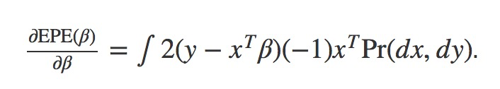
Before we proceed, let’s check the dimensions to make sure the partial derivative is correct. EPE is the expected error: a 1×1 vector. β is a column vector that is N×1. According to the Jacobian in vector calculus, the resulting partial derivative should take the form

which is a 1×N vector. Looking back at the right-hand side of the equation above, we find 2(y−xTβ)(−1) being a constant while xTbeing a row vector, resuling the same 1×Ndimension. Thus, we conclude the above partial derivative is correct. This derivative mirrors the relationship between the expected error and the way to adjust parameters so as to reduce the error. To understand why, imagine 2(y−xTβ)(−1) being the errors incurred by the current parameter configurations β and xT being the values of the input attributes. The resulting derivative equals to the error times the scales of each input attribute. Another way to make this point is: the contribution of error from each parameter βi has a monotonic relationship with the error 2(y−xTβ)(−1) as well as the scalar xT that was multiplied to each βi.
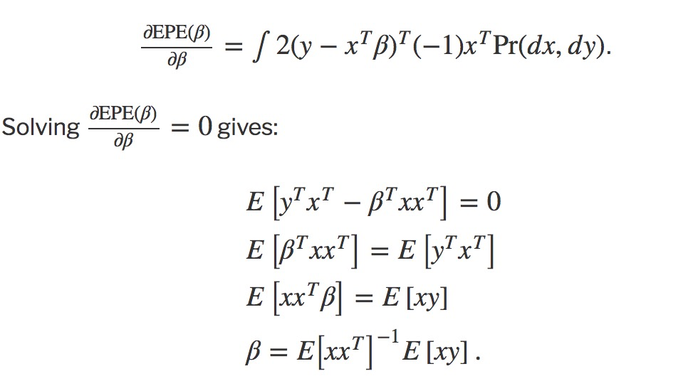
Now, let’s go back to the derivation. Because 2(y−xTβ)(−1) is 1×1, we can rewrite it with its transpose:
参考资料: