逻辑回归torch.nn实现

1 导入实验需要的包

import torch
from torch import nn
from torch.autograd import Variable
from torch.utils.data import DataLoader,TensorDataset
import matplotlib.pyplot as plt
import numpy as np
import os
os.environ["KMP_DUPLICATE_LIB_OK"]  =  "TRUE"

 

2 人工构造数据集

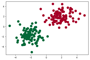
　　生成正/负样本各 50 个，特征数为2，进行二分类（0、1）.

# 假数据
n_data = torch.ones(100, 2)  # 数据的基本形态
x0 = torch.normal(2 * n_data, 1)  # 类型0 x data (tensor), shape=(100, 2)，好处共享均值和设置张量size
y0 = torch.zeros(100)  # 类型0 y data (tensor), shape=(100, 1)
x1 = torch.normal(-2 * n_data, 1)  # 类型1 x data (tensor), shape=(100, 1)
y1 = torch.ones(100)  # 类型1 y data (tensor), shape=(100, 1)


# 注意 x, y 数据的数据形式是一定要像下面一样 (torch.cat 是在合并数据)
x = torch.cat((x0, x1), 0).type(torch.FloatTensor)  # FloatTensor = 32-bit floating
y = torch.cat((y0, y1), 0).type(torch.FloatTensor)  # LongTensor = 64-bit integer

将两类样本用不同形状的标记表示出来，其中坐标轴是样本的两个特征。

plt.scatter(x.data.numpy()[:, 0], x.data.numpy()[:, 1], c=y.data.numpy(), s=100, lw=0, cmap='RdYlGn')
plt.show()

　　　　　　

3 定义模型

# class LogisticRegression(nn.Module):
#     def __init__(self):
#         super(LogisticRegression, self).__init__()
#         self.linear = nn.Linear(2, 1)
#         self.sm = nn.Sigmoid()

#     def forward(self, x):
#         x = self.lr(x)
#         x = self.sm(x)
#         return x
logistic_model =  nn.Sequential()
logistic_model.add_module('linear',nn.Linear(2,1))
logistic_model.add_module('sm',nn.Sigmoid())

# logistic_model = LogisticRegression()
if torch.cuda.is_available():
    logistic_model.cuda()

 

4 定义损失函数和优化器

# 定义损失函数和优化器
criterion = nn.BCELoss()
optimizer = torch.optim.SGD(logistic_model.parameters(), lr=1e-3, momentum=0.9)

 

5 随机打乱数据

　　感觉打乱无用，这一步。

# batch_size = 32
# data_iter = load_data(X,Y,batch_size)
def set_data(X,Y):
    index_slice = list(range(X.shape[0]))
    np.random.shuffle(index_slice)
    x =  X[index_slice]
    y =  Y[index_slice]
    if torch.cuda.is_available():
        x_data = Variable(x).cuda()
        y_data = Variable(y).cuda()
    else:
        x_data = Variable(x)
        y_data = Variable(y)
    return x_data,y_data

 

6 训练模型

Train_Loss_list = []
Train_acc_list = []

# 开始训练
for epoch in range(10000):
    x_data,y_data = set_data(x,y)
    out = logistic_model(x_data)
    out = out.view(-1,1)
    y_data = y_data.view(-1,1)
    loss = criterion(out, y_data)
    print_loss = loss.data.item()
    mask = out.ge(0.5).float()  # 以0.5为阈值进行分类
    correct = (mask == y_data).sum()  # 计算正确预测的样本个数
    acc = correct.item() / x_data.size(0)  # 计算精度
    optimizer.zero_grad()
    loss.backward()
    optimizer.step()
    Train_Loss_list.append(print_loss)
    Train_acc_list.append(acc)
    # 每隔2000轮打印一下当前的误差和精度
    if (epoch + 1) % 2000== 0:
        print('-' * 20)
        print('epoch {}'.format(epoch + 1))  # 训练轮数
        print('当前损失 {:.6f}'.format(print_loss))  # 误差
        print('当前精度 {:.6f}'.format(acc))  # 精度

结果：

--------------------
epoch 2000
当前损失 0.019348
当前精度 1.000000
--------------------
epoch 4000
当前损失 0.012090
当前精度 1.000000
--------------------
epoch 6000
当前损失 0.009251
当前精度 1.000000
--------------------
epoch 8000
当前损失 0.007668
当前精度 1.000000
--------------------
epoch 10000
当前损失 0.006634
当前精度 1.000000

输出模型参数值：

logistic_model.state_dict()

 结果：

　　OrderedDict([('linear.weight', tensor([[-2.1929, -1.9542]], device='cuda:0')), ('linear.bias', tensor([-0.2197], device='cuda:0'))])

7 绘制图表

x11= range(0,10000)
y11= Train_Loss_list
plt.xlabel('Train loss vs. epoches')
plt.ylabel('Train loss')
plt.plot(x11, y11,'.',c='b',label="Train_Loss")
plt.legend()
plt.show()

x11= range(0,10000)
y11= Train_acc_list
plt.xlabel('Train acc vs. epoches')
plt.ylabel('Train acc')
plt.plot(x11, y11,'.',c='b',label="Train_acc")
plt.legend()
plt.show()

结果：

　　　　　　

 

8 绘制分类结果图

# 结果可视化
w0, w1 = logistic_model.linear.weight[0]
w0 = float(w0.item())
w1 = float(w1.item())
b = float(logistic_model.linear.bias.item())
plot_x = np.arange(-7, 7, 0.1)
plot_y = (-w0 * plot_x - b) / w1
plt.scatter(x.data.numpy()[:, 0], x.data.numpy()[:, 1], c=y.data.numpy(), s=100, lw=0, cmap='RdYlGn')
plt.plot(plot_x, plot_y)
plt.show()

结果：