转自:http://yangl.net/2016/09/27/edger_usage/
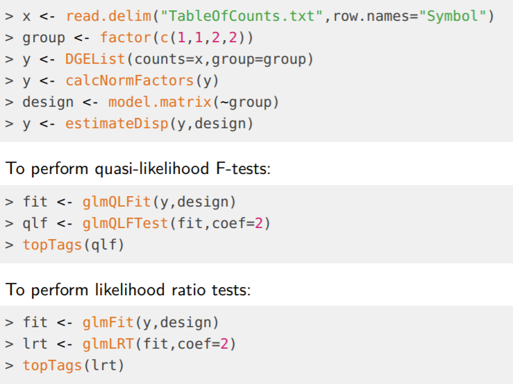
1.Quick start
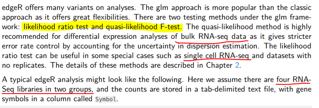
2. 利用edgeR分析RNA-seq鉴别差异表达基因:
#加载软件包
library("edgeR",verbose=0);

# 1. 载入数据 读取read count数
data <- read.delim("pnas_expression.txt", row.names=1, stringsAsFactors=FALSE);
head(data);

#输出
# lane1 lane2 lane3 lane4 lane5 lane6 lane8 len
# ENSG00000215696 0 0 0 0 0 0 0 330
# ENSG00000215700 0 0 0 0 0 0 0 2370
# ENSG00000215699 0 0 0 0 0 0 0 1842
# ENSG00000215784 0 0 0 0 0 0 0 2393
# ENSG00000212914 0 0 0 0 0 0 0 384
# ENSG00000212042 0 0 0 0 0 0 0 92

dim(data);
# [1] 37435 8

#2. 构建分组变量
#分为 Control组和DHT组 分别为4个和3个重复
targets <- data.frame(Lane = c(1:6,8), Treatment = c(rep("Control",4),rep("DHT",3)),
 Label = c(paste("Con", 1:4, sep=""), paste("DHT", 1:3, sep="")));

targets
#输出
# Lane Treatement Label
# 1 1 Control Con1
# 2 2 Control Con2
# 3 3 Control Con3
# 4 4 Control Con4
# 5 5 DHT DHT1
# 6 6 DHT DHT2
# 7 8 DHT DHT3

#3. 创建基因表达列表 进行标准化因子计算
y <- DGEList(counts=data[,1:7], group=targets$Treatment, genes=data.frame(Length=data[,8]));
colnames(y) <- targets$Label;
dim(y);
# [1] 37435 7


#过滤表达量偏低的基因 !!!
#基因在至少3个样本中得count per million(cpm)要大于1
keep <- rowSums(cpm(y)>1) >= 3;
y <- y[keep,];
dim(y)
# [1] 16494 7
#重新计算库大小
y$samples$lib.size <- colSums(y$counts);

#3. 进行标准化因子计算 默认使用TMM方法
y <- calcNormFactors(y);
y

#输出
# An object of class "DGEList"
# $counts
# Con1 Con2 Con3 Con4 DHT1 DHT2 DHT3
# ENSG00000124208 478 619 628 744 483 716 240
# ENSG00000182463 27 20 27 26 48 55 24
# ENSG00000124201 180 218 293 275 373 301 88
# ENSG00000124207 76 80 85 97 80 81 37
# ENSG00000125835 132 200 200 228 280 204 52
# 16489 more rows ...
#
# $samples
# group lib.size norm.factors
# Con1 1 976847 1.0296636
# Con2 1 1154746 1.0372521
# Con3 1 1439393 1.0362662
# Con4 1 1482652 1.0378383
# DHT1 1 1820628 0.9537095
# DHT2 1 1831553 0.9525624
# DHT3 1 680798 0.9583181
#
# $genes
# [1] 2131 5453 4060 3264 945
# 16489 more rows ...

#这里主要是通过图形的方式来展示实验组与对照组样本是否能明显的分开
#以及同一组内样本是否能聚的比较近 即重复样本是否具有一致性
plotMDS(y);


#4. 估计离散度
y <- estimateCommonDisp(y, verbose=TRUE)
# Disp = 0.02002 , BCV = 0.1415
y <- estimateTagwiseDisp(y);

plotBCV(y);

#5. 通过检验来鉴别差异表达基因
et <- exactTest(y);
top <- topTags(et);
top

#输出
# Comparison of groups: DHT-Control
# Length logFC logCPM PValue FDR
# ENSG00000151503 5605 5.816156 9.716866 0.000000e+00 0.000000e+00
# ENSG00000096060 4093 5.004454 9.950606 0.000000e+00 0.000000e+00
# ENSG00000166451 1556 4.683425 8.850401 2.297717e-249 1.263285e-245
# ENSG00000127954 3919 8.120955 7.216393 1.534440e-229 6.327264e-226
# ENSG00000162772 1377 3.316701 9.743797 7.975243e-216 2.630873e-212
# ENSG00000115648 2920 2.598440 11.474677 6.984860e-180 1.920138e-176
# ENSG00000116133 4286 3.244446 8.791930 1.290432e-174 3.040627e-171
# ENSG00000113594 10078 4.111120 8.055613 3.115276e-161 6.422921e-158
# ENSG00000130066 868 2.609899 9.989778 6.009018e-155 1.101253e-151
# ENSG00000116285 3076 4.201846 7.361640 6.299060e-149 1.038967e-145


#6. 定义差异表达基因与基本统计
summary(de <- decideTestsDGE(et)); # 默认选取FDR = 0.05为阈值

#输出
# [,1]
# -1 2094 #显著下调
# 0 12060 #没有显著差异
# 1 2340 #显著上调

#图形展示检验结果
detags <- rownames(y)[as.logical(de)];
plotSmear(et, de.tags=detags);
abline(h=c(-1, 1), col="blue");
//这个是分为 Control组和DHT组,检验这两组的差异表达基因。
//中间又一步是去除表达量过低的基因。
- 读取read count数
- 构建分组变量
- 创建基因表达列表 进行标准化因子计算 ,过滤表达量偏低的基因,进行标准化因子计算 默认使用TMM方法
- 估计离散度
- 通过检验来鉴别差异表达基因
- 定义差异表达基因与基本统计