0 - 学习目标
我们将实现一个简单的3层神经网络,我们不会仔细推到所需要的数学公式,但我们会给出我们这样做的直观解释。注意,此次代码并不能达到非常好的效果,可以自己进一步调整或者完成课后练习来进行改进。
1 - 实验步骤
1.1 - Import Packages
# Package imports
import matplotlib.pyplot as plt
import numpy as np
import sklearn
import sklearn.datasets
import sklearn.linear_model
import matplotlib

# Display plots inline and change default figure size
%matplotlib inline
matplotlib.rcParams['figure.figsize'] = (10.0, 8.0) # 指定matplotlib画布规模
1.2 - Generating a dataset
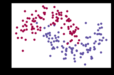
注意到,scikit-learn包包含了数据生成的代码,因此我们无需自己实现,直接采用其make_moons方法即可。下图中有两种类别的点,蓝点表示男患者,红点表示女患者,而xy坐标表示医学测量指标。我们的目的是去训练一个模型可以根据医学测量指标结果来划分男女患者,注意到图中的划分界限不是简单的线性的,因此采用简单的逻辑回归的效果合理不会很好。
# Generate a dataset and plot it
np.random.seed(0)
X, y = sklearn.datasets.make_moons(200, noise=0.20)
plt.scatter(X[:,0], X[:,1], s=40, c=y, cmap=plt.cm.Spectral)
1.3 - Logistic Regression
为了证明上述观点我们来训练一个逻辑回归模型看看效果。输入是xy坐标,而输出是(0,1)二分类。我们直接使用scikit-learn包中的逻辑回归算法做预测。
# Train the logistic regression classifier
clf = sklearn.linear_model.LogisticRegressionCV()
clf.fit(X, y)
Out[3]:
LogisticRegressionCV(Cs=10, class_weight=None, cv=None, dual=False,
           fit_intercept=True, intercept_scaling=1.0, max_iter=100,
           multi_class='ovr', n_jobs=1, penalty='l2', random_state=None,
           refit=True, scoring=None, solver='lbfgs', tol=0.0001, verbose=0)
# Helper function to plot a decision boundary.
# If you don't fully understand this function don't worry, it just generates the contour plot below.
def plot_decision_boundary(pred_func):
    # Set min and max values and give it some padding
    x_min, x_max = X[:, 0].min() - .5, X[:, 0].max() + .5
    y_min, y_max = X[:, 1].min() - .5, X[:, 1].max() + .5
    h = 0.01
    # Generate a grid of points with distance h between them
    xx, yy = np.meshgrid(np.arange(x_min, x_max, h), np.arange(y_min, y_max, h))
    # Predict the function value for the whole gid
    Z = pred_func(np.c_[xx.ravel(), yy.ravel()])
    Z = Z.reshape(xx.shape)
    # Plot the contour and training examples
    plt.contourf(xx, yy, Z, cmap=plt.cm.Spectral)
    plt.scatter(X[:, 0], X[:, 1], c=y, cmap=plt.cm.Spectral)
# Plot the decision boundary
plot_decision_boundary(lambda x: clf.predict(x))
plt.title("Logistic Regression")
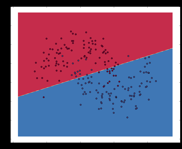
可以看到,逻辑回归使用一条直线尽可能好的分割这个二分类问题,但是由于原先数据本就不是线性可分的,因此效果并不好。
1.4 - Training a Neural Network
现在来构建一个有一个输入层一个隐藏层和一个输出层的简单三层神经网络来做预测。
1.4.1 - How our network makes predictions
神经网络通过下述公式进行预测。
$$
\begin{aligned}
z_1 & = xW_1 + b_1 \\
a_1 & = \tanh(z_1) \\
z_2 & = a_1W_2 + b_2 \\
a_2 & = \hat{y} = \mathrm{softmax}(z_2)
\end{aligned}
$$
1.4.2 - Learning the Parameters
学习参数是让我们的网络找到一组参数 ($W_1, b_1, W_2, b_2$)使得训练集上的损失最小化。现在我们来定义损失函数,这里我们使用常用的交叉熵损失函数,如下:
$$
\begin{aligned}
L(y,\hat{y}) = - \frac{1}{N} \sum_{n \in N} \sum_{i \in C} y_{n,i} \log\hat{y}_{n,i}
\end{aligned}
$$
而后我们使用梯度下降来最小化损失函数。我们将实现最简单的梯度下降算法,其实就是有着固定学习率的批量梯度下降。在实践中,梯度下降的一些变种如SGD(随机梯度下降)或者最小批次梯度下降往往有更好的表现。因此后续我们可以通过这些点来改进效果。
梯度下降需要计算出损失函数相对于我们要更新参数的梯度 $\frac{\partial{L}}{\partial{W_1}}$, $\frac{\partial{L}}{\partial{b_1}}$, $\frac{\partial{L}}{\partial{W_2}}$, $\frac{\partial{L}}{\partial{b_2}}$。为了计算这些梯度我们使用著名的反向传播算法,这种方法能够从输出开始有效地计算梯度。此处不细讲反向传播是如何工作的,只给出方向传播需要的公式,如下:
$$
\begin{aligned}
& \delta_3 = \hat{y} - y \\
& \delta_2 = (1 - \tanh^2z_1) \circ \delta_3W_2^T \\
& \frac{\partial{L}}{\partial{W_2}} = a_1^T \delta_3 \\
& \frac{\partial{L}}{\partial{b_2}} = \delta_3\\
& \frac{\partial{L}}{\partial{W_1}} = x^T \delta_2\\
& \frac{\partial{L}}{\partial{b_1}} = \delta_2 \\
\end{aligned}
$$
1.4.3 - Implementation
开始实现!
变量定义。
num_examples = len(X) # 训练集大小
nn_input_dim = 2 # 输入层维度
nn_output_dim = 2 # 输出层维度

# Gradient descent parameters (I picked these by hand)
epsilon = 0.01 # 梯度下降学习率
reg_lambda = 0.01 # 正规化权重
损失函数定义。
# Helper function to evaluate the total loss on the dataset
def calculate_loss(model):
    W1, b1, W2, b2 = model['W1'], model['b1'], model['W2'], model['b2']
    # 前向传播,计算出预测值
    z1 = X.dot(W1) + b1
    a1 = np.tanh(z1)
    z2 = a1.dot(W2) + b2
    exp_scores = np.exp(z2)
    probs = exp_scores / np.sum(exp_scores, axis=1, keepdims=True)
    # 计算损失
    corect_logprobs = -np.log(probs[range(num_examples), y])
    data_loss = np.sum(corect_logprobs)
    # 损失值加入正规化
    data_loss += reg_lambda/2 * (np.sum(np.square(W1)) + np.sum(np.square(W2)))
    return 1./num_examples * data_loss
我们也实现了一个有用的用来计算网络输出的方法,其做了前向传播计算并且返回最高概率类别。
# Helper function to predict an output (0 or 1)
def predict(model, x):
    W1, b1, W2, b2 = model['W1'], model['b1'], model['W2'], model['b2']
    # Forward propagation
    z1 = x.dot(W1) + b1
    a1 = np.tanh(z1)
    z2 = a1.dot(W2) + b2
    exp_scores = np.exp(z2)
    probs = exp_scores / np.sum(exp_scores, axis=1, keepdims=True)
    return np.argmax(probs, axis=1)
最后,使用批量梯度下降算法来训练我们的神经网络。
# This function learns parameters for the neural network and returns the model.
# - nn_hdim: Number of nodes in the hidden layer
# - num_passes: Number of passes through the training data for gradient descent
# - print_loss: If True, print the loss every 1000 iterations
def build_model(nn_hdim, num_passes=20000, print_loss=False):

    # 随机初始化权重
    np.random.seed(0)
    W1 = np.random.randn(nn_input_dim, nn_hdim) / np.sqrt(nn_input_dim)
    b1 = np.zeros((1, nn_hdim))
    W2 = np.random.randn(nn_hdim, nn_output_dim) / np.sqrt(nn_hdim)
    b2 = np.zeros((1, nn_output_dim))

    # 返回字典初始化
    model = {}

    # 对于每一个批次进行梯度下降
    for i in range(0, num_passes):

        # 前向传播
        z1 = X.dot(W1) + b1
        a1 = np.tanh(z1)
        z2 = a1.dot(W2) + b2
        exp_scores = np.exp(z2)
        probs = exp_scores / np.sum(exp_scores, axis=1, keepdims=True)

        # 反向传播
        delta3 = probs
        delta3[range(num_examples), y] -= 1
        dW2 = (a1.T).dot(delta3)
        db2 = np.sum(delta3, axis=0, keepdims=True)
        delta2 = delta3.dot(W2.T) * (1 - np.power(a1, 2))
        dW1 = np.dot(X.T, delta2)
        db1 = np.sum(delta2, axis=0)

        # 加入正则化
        dW2 += reg_lambda * W2
        dW1 += reg_lambda * W1

        # 梯度下降参数更新
        W1 += -epsilon * dW1
        b1 += -epsilon * db1
        W2 += -epsilon * dW2
        b2 += -epsilon * db2

        # 分配新权重
        model = { 'W1': W1, 'b1': b1, 'W2': W2, 'b2': b2}

        # Optionally print the loss.
        # This is expensive because it uses the whole dataset, so we don't want to do it too often.
        if print_loss and i % 1000 == 0:
          print("Loss after iteration %i: %f" %(i, calculate_loss(model)))

    return model
1.4.4 - A network with a hidden layer of size 3
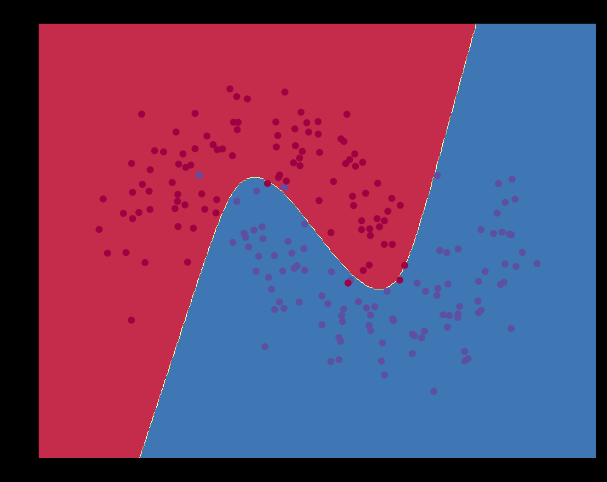
# Build a model with a 3-dimensional hidden layer
model = build_model(3, print_loss=True)

# Plot the decision boundary
plot_decision_boundary(lambda x: predict(model, x))
plt.title("Decision Boundary for hidden layer size 3")
Loss after iteration 0: 0.432387
Loss after iteration 1000: 0.068947
Loss after iteration 2000: 0.068926
Loss after iteration 3000: 0.071218
Loss after iteration 4000: 0.071253
Loss after iteration 5000: 0.071278
Loss after iteration 6000: 0.071293
Loss after iteration 7000: 0.071303
Loss after iteration 8000: 0.071308
Loss after iteration 9000: 0.071312
Loss after iteration 10000: 0.071314
Loss after iteration 11000: 0.071315
Loss after iteration 12000: 0.071315
Loss after iteration 13000: 0.071316
Loss after iteration 14000: 0.071316
Loss after iteration 15000: 0.071316
Loss after iteration 16000: 0.071316
Loss after iteration 17000: 0.071316
Loss after iteration 18000: 0.071316
Loss after iteration 19000: 0.071316

这看起来比逻辑回归的效果好多了!
1.5 - Varying the hidden layer size
plt.figure(figsize=(16, 32))
hidden_layer_dimensions = [1, 2, 3, 4, 5, 20, 50]
for i, nn_hdim in enumerate(hidden_layer_dimensions):
    plt.subplot(5, 2, i+1)
    plt.title('Hidden Layer size %d' % nn_hdim)
    model = build_model(nn_hdim)
    plot_decision_boundary(lambda x: predict(model, x))
plt.show()

2 - Exercises
我们给出了一些练习。
- Instead of batch gradient descent, use minibatch gradient descent (more info) to train the network. Minibatch gradient descent typically performs better in practice.
- We used a fixed learning rate $\epsilon$ for gradient descent. Implement an annealing schedule for the gradient descent learning rate (more info).
- We used a $\tanh$ activation function for our hidden layer. Experiment with other activation functions (some are mentioned above). Note that changing the activation function also means changing the backpropagation derivative.
- Extend the network from two to three classes. You will need to generate an appropriate dataset for this.
- Extend the network to four layers. Experiment with the layer size. Adding another hidden layer means you will need to adjust both the forward propagation as well as the backpropagation code.
3 - Exercises (1)
采用随机梯度下降方法,由于本题我是在第五题之后写的,因此采用的还是第五题构造的四层网络结构。
重写build_model,如下:
# This function learns parameters for the neural network and returns the model.
# - nn_hdim1: Number of nodes in the first hidden layer
# - nn_hidm2: Number of nodes in the second hidden layer(default 3)
# - m: Size of minibatch
# - num_passes: Number of passes through the training data for gradient descent
# - print_loss: If True, print the loss every 1000 iterations
# - d: the decay number of annealing schedule
def build_model(nn_hdim1, nn_hdim2=3, m=128, num_passes=20000, print_loss=False, d=10e-3):

    # Initialize the parameters to random values. We need to learn these.
    np.random.seed(0)
    W1 = np.random.randn(nn_input_dim, nn_hdim1) / np.sqrt(nn_input_dim)
    b1 = np.zeros((1, nn_hdim1))
    W2 = np.random.randn(nn_hdim1, nn_hdim2) / np.sqrt(nn_hdim1)
    b2 = np.zeros((1, nn_hdim2))
    W3 = np.random.randn(nn_hdim2, nn_output_dim) / np.sqrt(nn_hdim2)
    b3 = np.zeros((1, nn_output_dim))

    # This is what we return at the end
    model = {}

    # Gradient descent. For each batch...
    for i in range(0, num_passes):

        X_length = len(X)
        import random
        index = random.sample(range(0,X_length), m)
        X_ = X[index]
        y_ = y[index]
        # Forward propagation
        z1 = X_.dot(W1) + b1
        a1 = sigmoid(z1)
        z2 = a1.dot(W2) + b2
        a2 = sigmoid(z2)
        z3 = a2.dot(W3) + b3
        exp_scores = np.exp(z3)
        probs = exp_scores / np.sum(exp_scores, axis=1, keepdims=True)

        # Backpropagation
        delta4 = probs
        delta4[range(m), y_] -= 1
        dW3 = (a2.T).dot(delta4)
        db3 = np.sum(delta4, axis=0, keepdims=True)
        delta3 = delta4.dot(W3.T) * a2 * (1-a2)
        dW2 = np.dot(a1.T, delta3)
        db2 = np.sum(delta3, axis=0)
        delta2 = delta3.dot(W2.T) * a1 * (1-a1)
        dW1 = np.dot(X_.T, delta2)
        db1 = np.sum(delta2, axis=0)

        # Add regularization terms (b1 and b2 don't have regularization terms)
        dW3 += reg_lambda * W3
        dW2 += reg_lambda * W2
        dW1 += reg_lambda * W1

        epsilon_ = epsilon / (1+d*i)
        # Gradient descent parameter update
        W1 += -epsilon_ * dW1
        b1 += -epsilon_ * db1
        W2 += -epsilon_ * dW2
        b2 += -epsilon_ * db2
        W3 += -epsilon_ * dW3
        b3 += -epsilon_ * db3

        # Assign new parameters to the model
        model = { 'W1': W1, 'b1': b1, 'W2': W2, 'b2': b2, 'W3': W3, 'b3': b3}

        # Optionally print the loss.
        # This is expensive because it uses the whole dataset, so we don't want to do it too often.
        if print_loss and i % 1000 == 0:
          print("Loss after iteration %i: %f" %(i, calculate_loss(model)))

    return model
结果:
Loss after iteration 0: 0.690824
Loss after iteration 1000: 0.303296
Loss after iteration 2000: 0.282995
Loss after iteration 3000: 0.255683
Loss after iteration 4000: 0.229780
Loss after iteration 5000: 0.208478
Loss after iteration 6000: 0.191594
Loss after iteration 7000: 0.178304
Loss after iteration 8000: 0.167675
Loss after iteration 9000: 0.159266
Loss after iteration 10000: 0.152439
Loss after iteration 11000: 0.146777
Loss after iteration 12000: 0.142068
Loss after iteration 13000: 0.138093
Loss after iteration 14000: 0.134683
Loss after iteration 15000: 0.131718
Loss after iteration 16000: 0.129113
Loss after iteration 17000: 0.126861
Loss after iteration 18000: 0.124822
Loss after iteration 19000: 0.123014

可以看到,当随机梯度的$minibatch$的大小设置为128时,效果并不如批量梯度下降。但是$minibatch$的效率明显比批量梯度下降高,而且如果进行更多轮的迭代效果也很有可能变好,这也是现在训练神经网络更多的采用$minibatch$梯度下降的原因。
4 - Exercises (2)
使用模拟退火算法更新学习率,公式为$epsilon=\frac{epsilon_0}{1+d \times t}$。
# This function learns parameters for the neural network and returns the model.
# - nn_hdim: Number of nodes in the hidden layer
# - num_passes: Number of passes through the training data for gradient descent
# - print_loss: If True, print the loss every 1000 iterations
# - d: the decay number of annealing schedule
def build_model(nn_hdim, num_passes=20000, print_loss=False, d=10e-3):

    # Initialize the parameters to random values. We need to learn these.
    np.random.seed(0)
    W1 = np.random.randn(nn_input_dim, nn_hdim) / np.sqrt(nn_input_dim)
    b1 = np.zeros((1, nn_hdim))
    W2 = np.random.randn(nn_hdim, nn_output_dim) / np.sqrt(nn_hdim)
    b2 = np.zeros((1, nn_output_dim))

    # This is what we return at the end
    model = {}

    # Gradient descent. For each batch...
    for i in range(0, num_passes):

        # Forward propagation
        z1 = X.dot(W1) + b1
        a1 = np.tanh(z1)
        z2 = a1.dot(W2) + b2
        exp_scores = np.exp(z2)
        probs = exp_scores / np.sum(exp_scores, axis=1, keepdims=True)

        # Backpropagation
        delta3 = probs
        delta3[range(num_examples), y] -= 1
        dW2 = (a1.T).dot(delta3)
        db2 = np.sum(delta3, axis=0, keepdims=True)
        delta2 = delta3.dot(W2.T) * (1 - np.power(a1, 2))
        dW1 = np.dot(X.T, delta2)
        db1 = np.sum(delta2, axis=0)

        # Add regularization terms (b1 and b2 don't have regularization terms)
        dW2 += reg_lambda * W2
        dW1 += reg_lambda * W1

        epsilon_ = epsilon / (1+d*i)
        # Gradient descent parameter update
        W1 += -epsilon_ * dW1
        b1 += -epsilon_ * db1
        W2 += -epsilon_ * dW2
        b2 += -epsilon_ * db2

        # Assign new parameters to the model
        model = { 'W1': W1, 'b1': b1, 'W2': W2, 'b2': b2}

        # Optionally print the loss.
        # This is expensive because it uses the whole dataset, so we don't want to do it too often.
        if print_loss and i % 1000 == 0:
          print("Loss after iteration %i: %f" %(i, calculate_loss(model)))

    return model
Loss after iteration 0: 0.432387
Loss after iteration 1000: 0.081007
Loss after iteration 2000: 0.075384
Loss after iteration 3000: 0.073729
Loss after iteration 4000: 0.072895
Loss after iteration 5000: 0.072376
Loss after iteration 6000: 0.072013
Loss after iteration 7000: 0.071742
Loss after iteration 8000: 0.071530
Loss after iteration 9000: 0.071357
Loss after iteration 10000: 0.071214
Loss after iteration 11000: 0.071092
Loss after iteration 12000: 0.070986
Loss after iteration 13000: 0.070894
Loss after iteration 14000: 0.070812
Loss after iteration 15000: 0.070739
Loss after iteration 16000: 0.070673
Loss after iteration 17000: 0.070613
Loss after iteration 18000: 0.070559
Loss after iteration 19000: 0.070509
4 - Exercises (3)
改用激活函数,由于本题我是在第五题之后写的,因此采用的还是第五题构造的四层网络结构,我决定采用$sigmoid$函数替代$tanh$函数做激活函数,其介绍可见于我的另一篇博客sigmoid理解。因此,反向传播公式需要重新推导,结果如下:
$$
\begin{aligned}
& \delta_4 = \hat{y} - y \\
& \delta_3 = sigmoid(x)(1-sigmoid(x)) \circ \delta_4W_3^T \\
& \delta_2 = sigmoid(x)(1-sigmoid(x)) \circ \delta_3W_2^T \\
& \frac{\partial{L}}{\partial{W_3}} = a_2^T \delta_4 \\
& \frac{\partial{L}}{\partial{b_3}} = \delta_4\\
& \frac{\partial{L}}{\partial{W_2}} = a_1^T \delta_3\\
& \frac{\partial{L}}{\partial{b_2}} = \delta_3 \\
& \frac{\partial{L}}{\partial{W_1}} = x^T \delta_2 \\
& \frac{\partial{L}}{\partial{b_1}} = \delta_2 \\
\end{aligned}
$$
定义$sigmoid$函数,如下:
def sigmoid(x):
    return 1 / (1 + np.exp(-x))
重写calculate_loss方法,如下:
# Helper function to evaluate the total loss on the dataset
def calculate_loss(model):
    W1, b1, W2, b2, W3, b3 = model['W1'], model['b1'], model['W2'], model['b2'], model['W3'], model['b3']
    # Forward propagation to calculate our predictions
    z1 = X.dot(W1) + b1
    a1 = sigmoid(z1)
    z2 = a1.dot(W2) + b2
    a2 = sigmoid(z2)
    z3 = a2.dot(W3) + b3
    exp_scores = np.exp(z3)
    probs = exp_scores / np.sum(exp_scores, axis=1, keepdims=True)
    # Calculating the loss
    corect_logprobs = -np.log(probs[range(num_examples), y])
    data_loss = np.sum(corect_logprobs)
    # Add regulatization term to loss (optional)
    data_loss += reg_lambda/2 * (np.sum(np.square(W1)) + np.sum(np.square(W2)))
    return 1./num_examples * data_loss
重写predict方法,如下:
# Helper function to predict an output (0 or 1)
def predict(model, x):
    W1, b1, W2, b2, W3, b3 = model['W1'], model['b1'], model['W2'], model['b2'], model['W3'], model['b3']
    # Forward propagation
    z1 = x.dot(W1) + b1
    a1 = sigmoid(z1)
    z2 = a1.dot(W2) + b2
    a2 = sigmoid(z2)
    z3 = a2.dot(W3) + b3
    exp_scores = np.exp(z3)
    probs = exp_scores / np.sum(exp_scores, axis=1, keepdims=True)
    return np.argmax(probs, axis=1)
重写build_model方法,如下:
# This function learns parameters for the neural network and returns the model.
# - nn_hdim1: Number of nodes in the first hidden layer
# - nn_hidm2: Number of nodes in the second hidden layer(default 3)
# - num_passes: Number of passes through the training data for gradient descent
# - print_loss: If True, print the loss every 1000 iterations
# - d: the decay number of annealing schedule
def build_model(nn_hdim1, nn_hdim2=3, num_passes=20000, print_loss=False, d=10e-3):

    # Initialize the parameters to random values. We need to learn these.
    np.random.seed(0)
    W1 = np.random.randn(nn_input_dim, nn_hdim1) / np.sqrt(nn_input_dim)
    b1 = np.zeros((1, nn_hdim1))
    W2 = np.random.randn(nn_hdim1, nn_hdim2) / np.sqrt(nn_hdim1)
    b2 = np.zeros((1, nn_hdim2))
    W3 = np.random.randn(nn_hdim2, nn_output_dim) / np.sqrt(nn_hdim2)
    b3 = np.zeros((1, nn_output_dim))

    # This is what we return at the end
    model = {}

    # Gradient descent. For each batch...
    for i in range(0, num_passes):

        # Forward propagation
        z1 = X.dot(W1) + b1
        a1 = sigmoid(z1)
        z2 = a1.dot(W2) + b2
        a2 = sigmoid(z2)
        z3 = a2.dot(W3) + b3
        exp_scores = np.exp(z3)
        probs = exp_scores / np.sum(exp_scores, axis=1, keepdims=True)

        # Backpropagation
        delta4 = probs
        delta4[range(num_examples), y] -= 1
        dW3 = (a2.T).dot(delta4)
        db3 = np.sum(delta4, axis=0, keepdims=True)
        delta3 = delta4.dot(W3.T) * a2 * (1-a2)
        dW2 = np.dot(a1.T, delta3)
        db2 = np.sum(delta3, axis=0)
        delta2 = delta3.dot(W2.T) * a1 * (1-a1)
        dW1 = np.dot(X.T, delta2)
        db1 = np.sum(delta2, axis=0)

        # Add regularization terms (b1 and b2 don't have regularization terms)
        dW3 += reg_lambda * W3
        dW2 += reg_lambda * W2
        dW1 += reg_lambda * W1

        epsilon_ = epsilon / (1+d*i)
        # Gradient descent parameter update
        W1 += -epsilon_ * dW1
        b1 += -epsilon_ * db1
        W2 += -epsilon_ * dW2
        b2 += -epsilon_ * db2
        W3 += -epsilon_ * dW3
        b3 += -epsilon_ * db3

        # Assign new parameters to the model
        model = { 'W1': W1, 'b1': b1, 'W2': W2, 'b2': b2, 'W3': W3, 'b3': b3}

        # Optionally print the loss.
        # This is expensive because it uses the whole dataset, so we don't want to do it too often.
        if print_loss and i % 1000 == 0:
          print("Loss after iteration %i: %f" %(i, calculate_loss(model)))

    return model
结果:
Loss after iteration 0: 0.685280
Loss after iteration 1000: 0.221651
Loss after iteration 2000: 0.140964
Loss after iteration 3000: 0.117482
Loss after iteration 4000: 0.107298
Loss after iteration 5000: 0.101436
Loss after iteration 6000: 0.097515
Loss after iteration 7000: 0.094664
Loss after iteration 8000: 0.092479
Loss after iteration 9000: 0.090744
Loss after iteration 10000: 0.089330
Loss after iteration 11000: 0.088153
Loss after iteration 12000: 0.087156
Loss after iteration 13000: 0.086301
Loss after iteration 14000: 0.085559
Loss after iteration 15000: 0.084907
Loss after iteration 16000: 0.084331
Loss after iteration 17000: 0.083816
Loss after iteration 18000: 0.083354
Loss after iteration 19000: 0.082936
由上可以看到,换成$sigmoid$激活函数的效果其实反而不如$tanh$激活函数。但现在神经网络常用的还是$sigmoid$激活函数,具体原因后续我将再写博客进行分析。总之不能以偏概全,在这个小实验中还有很多其他的参数也会影响到结果,因此不能绝对的说$sigmoid$就必定好于$tanh$!
5 - Exercises (4)
将网络的识别类别从两类扩充到三类,只需要修改变量nn_output_dim为3即可。由于没有找到合适的三分类数据集,因此不做测试。
6 - Exercises (5)
将网络扩展到四层,则反向传播公式如下(其中关于tanh激活函数见于我的另一篇博客tanh理解,DNN的反向传播算法理解见于我的另一篇博客DNN反向传播):
$$
\begin{aligned}
& \delta_4 = \hat{y} - y \\
& \delta_3 = (1 - \tanh^2z_2) \circ \delta_4W_3^T \\
& \delta_2 = (1 - \tanh^2z_1) \circ \delta_3W_2^T \\
& \frac{\partial{L}}{\partial{W_3}} = a_2^T \delta_4 \\
& \frac{\partial{L}}{\partial{b_3}} = \delta_4\\
& \frac{\partial{L}}{\partial{W_2}} = a_1^T \delta_3\\
& \frac{\partial{L}}{\partial{b_2}} = \delta_3 \\
& \frac{\partial{L}}{\partial{W_1}} = x^T \delta_2 \\
& \frac{\partial{L}}{\partial{b_1}} = \delta_2 \\
\end{aligned}
$$
重写calculate_loss方法如下:
# Helper function to evaluate the total loss on the dataset
def calculate_loss(model):
    W1, b1, W2, b2, W3, b3 = model['W1'], model['b1'], model['W2'], model['b2'], model['W3'], model['b3']
    # Forward propagation to calculate our predictions
    z1 = X.dot(W1) + b1
    a1 = np.tanh(z1)
    z2 = a1.dot(W2) + b2
    a2 = np.tanh(z2)
    z3 = a2.dot(W3) + b3
    exp_scores = np.exp(z3)
    probs = exp_scores / np.sum(exp_scores, axis=1, keepdims=True)
    # Calculating the loss
    corect_logprobs = -np.log(probs[range(num_examples), y])
    data_loss = np.sum(corect_logprobs)
    # Add regulatization term to loss (optional)
    data_loss += reg_lambda/2 * (np.sum(np.square(W1)) + np.sum(np.square(W2)))
    return 1./num_examples * data_loss
重写predict方法如下:
# Helper function to predict an output (0 or 1)
def predict(model, x):
    W1, b1, W2, b2, W3, b3 = model['W1'], model['b1'], model['W2'], model['b2'], model['W3'], model['b3']
    # Forward propagation
    z1 = x.dot(W1) + b1
    a1 = np.tanh(z1)
    z2 = a1.dot(W2) + b2
    a2 = np.tanh(z2)
    z3 = a2.dot(W3) + b3
    exp_scores = np.exp(z3)
    probs = exp_scores / np.sum(exp_scores, axis=1, keepdims=True)
    return np.argmax(probs, axis=1)
重写build_model方法如下:
# This function learns parameters for the neural network and returns the model.
# - nn_hdim1: Number of nodes in the first hidden layer
# - nn_hidm2: Number of nodes in the second hidden layer(default 3)
# - num_passes: Number of passes through the training data for gradient descent
# - print_loss: If True, print the loss every 1000 iterations
# - d: the decay number of annealing schedule
def build_model(nn_hdim1, nn_hdim2=3, num_passes=20000, print_loss=False, d=10e-3):

    # Initialize the parameters to random values. We need to learn these.
    np.random.seed(0)
    W1 = np.random.randn(nn_input_dim, nn_hdim1) / np.sqrt(nn_input_dim)
    b1 = np.zeros((1, nn_hdim1))
    W2 = np.random.randn(nn_hdim1, nn_hdim2) / np.sqrt(nn_hdim1)
    b2 = np.zeros((1, nn_hdim2))
    W3 = np.random.randn(nn_hdim2, nn_output_dim) / np.sqrt(nn_hdim2)
    b3 = np.zeros((1, nn_output_dim))

    # This is what we return at the end
    model = {}

    # Gradient descent. For each batch...
    for i in range(0, num_passes):

        # Forward propagation
        z1 = X.dot(W1) + b1
        a1 = np.tanh(z1)
        z2 = a1.dot(W2) + b2
        a2 = np.tanh(z2)
        z3 = a2.dot(W3) + b3
        exp_scores = np.exp(z3)
        probs = exp_scores / np.sum(exp_scores, axis=1, keepdims=True)

        # Backpropagation
        delta4 = probs
        delta4[range(num_examples), y] -= 1
        dW3 = (a2.T).dot(delta4)
        db3 = np.sum(delta4, axis=0, keepdims=True)
        delta3 = delta4.dot(W3.T) * (1 - np.power(a2, 2))
        dW2 = np.dot(a1.T, delta3)
        db2 = np.sum(delta3, axis=0)
        delta2 = delta3.dot(W2.T) * (1 - np.power(a1, 2))
        dW1 = np.dot(X.T, delta2)
        db1 = np.sum(delta2, axis=0)

        # Add regularization terms (b1 and b2 don't have regularization terms)
        dW3 += reg_lambda * W3
        dW2 += reg_lambda * W2
        dW1 += reg_lambda * W1

        epsilon_ = epsilon / (1+d*i)
        # Gradient descent parameter update
        W1 += -epsilon_ * dW1
        b1 += -epsilon_ * db1
        W2 += -epsilon_ * dW2
        b2 += -epsilon_ * db2
        W3 += -epsilon_ * dW3
        b3 += -epsilon_ * db3

        # Assign new parameters to the model
        model = { 'W1': W1, 'b1': b1, 'W2': W2, 'b2': b2, 'W3': W3, 'b3': b3}

        # Optionally print the loss.
        # This is expensive because it uses the whole dataset, so we don't want to do it too often.
        if print_loss and i % 1000 == 0:
          print("Loss after iteration %i: %f" %(i, calculate_loss(model)))

    return model
效果:
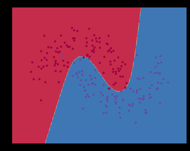
可以看到四层的结果比三层好(loss小了)。
7 - 参考资料
http://www.wildml.com/2015/09/implementing-a-neural-network-from-scratch/
https://github.com/dennybritz/nn-from-scratch
https://www.cnblogs.com/CZiFan/p/9474615.html