目录
import keras
keras.__version__
Using TensorFlow backend.

'2.3.1'
Predicting house prices: a regression example
This notebook contains the code samples found in Chapter 3, Section 6 of Deep Learning with Python. Note that the original text features far more content, in particular further explanations and figures: in this notebook, you will only find source code and related comments.
In our two previous examples, we were considering classification problems, where the goal was to predict a single discrete label of an
input data point. Another common type of machine learning problem is “regression”, which consists of predicting a continuous value instead
of a discrete label. For instance, predicting the temperature tomorrow, given meteorological data, or predicting the time that a
software project will take to complete, given its specifications.
Do not mix up “regression” with the algorithm “logistic regression”: confusingly, “logistic regression” is not a regression algorithm,
it is a classification algorithm.
预测房价:回归问题
前面两个例子都是分类问题,其目标是预测输入数据点所对应的单一离散的标签。另一种常见的机器学习问题是回归问题,它预测一个连续值而不是离散的标签,例如,根据气象数据预测明天的气温,或者根据软件说明书预测完成软件项目所需要的时间。
The Boston Housing Price dataset
We will be attempting to predict the median price of homes in a given Boston suburb in the mid-1970s, given a few data points about the
suburb at the time, such as the crime rate, the local property tax rate, etc.
The dataset we will be using has another interesting difference from our two previous examples: it has very few data points, only 506 in
total, split between 404 training samples and 102 test samples, and each “feature” in the input data (e.g. the crime rate is a feature) has
a different scale. For instance some values are proportions, which take a values between 0 and 1, others take values between 1 and 12,
others between 0 and 100…
Let’s take a look at the data:
波士顿房价数据集
本节将要预测 20 世纪 70 年代中期波士顿郊区房屋价格的中位数,已知当时郊区的一些数据点,比如犯罪率、当地房产税率等。
本节用到的数据集与前面两个例子有一个有趣的区别。它包含的数据点相对较少,只有 506 个,分为 404 个训练样本和 102 个测试样本。输入数据的每个特征(比如犯罪率)都有不同的取值范围。例如,有些特性是比例,取值范围为 0~1;有的取值范围为 1~12;还有的取值范围为 0~100,等等。
from keras.datasets import boston_housing

(train_data, train_targets), (test_data, test_targets) =  boston_housing.load_data()
train_data.shape
(404, 13)
test_data.shape
(102, 13)
As you can see, we have 404 training samples and 102 test samples. The data comprises 13 features. The 13 features in the input data are as
follow:
- Per capita crime rate.
- Proportion of residential land zoned for lots over 25,000 square feet.
- Proportion of non-retail business acres per town.
- Charles River dummy variable (= 1 if tract bounds river; 0 otherwise).
- Nitric oxides concentration (parts per 10 million).
- Average number of rooms per dwelling.
- Proportion of owner-occupied units built prior to 1940.
- Weighted distances to five Boston employment centres.
- Index of accessibility to radial highways.
- Full-value property-tax rate per $10,000.
- Pupil-teacher ratio by town.
- 1000 * (Bk - 0.63) ** 2 where Bk is the proportion of Black people by town.
- % lower status of the population.
The targets are the median values of owner-occupied homes, in thousands of dollars:
如您所见,我们有404个训练样本和102个测试样本。 数据包含13个特征。 输入数据中的13个特征如下:
- 人均犯罪率。
- 占地超过25,000平方英尺的住宅用地比例。
- 每个镇非零售业务用地的比例。
- 查尔斯河虚拟变量(如果束缚河流,则为1;否则为0)。
- 一氧化氮浓度(百万分之几)。
- 每个住宅的平均房间数。
- 1940年以前建造的自有住房的比例。
- 到五个波士顿就业中心的加权距离。
- 径向公路的可达性指数。
- 每$ 10,000美元的全值财产税率。
- 各镇的师生比例。
- 1000 (Bk-0.63)* 2其中,Bk是按城镇划分的黑人比例。
- 人口状况下降13.%。
目标是自住房价格的中位数,以千美元为单位:
train_targets
array([15.2, 42.3, 50. , 21.1, 17.7, 18.5, 11.3, 15.6, 15.6, 14.4, 12.1,
       17.9, 23.1, 19.9, 15.7,  8.8, 50. , 22.5, 24.1, 27.5, 10.9, 30.8,
       32.9, 24. , 18.5, 13.3, 22.9, 34.7, 16.6, 17.5, 22.3, 16.1, 14.9,
       23.1, 34.9, 25. , 13.9, 13.1, 20.4, 20. , 15.2, 24.7, 22.2, 16.7,
       12.7, 15.6, 18.4, 21. , 30.1, 15.1, 18.7,  9.6, 31.5, 24.8, 19.1,
       22. , 14.5, 11. , 32. , 29.4, 20.3, 24.4, 14.6, 19.5, 14.1, 14.3,
       15.6, 10.5,  6.3, 19.3, 19.3, 13.4, 36.4, 17.8, 13.5, 16.5,  8.3,
       14.3, 16. , 13.4, 28.6, 43.5, 20.2, 22. , 23. , 20.7, 12.5, 48.5,
       14.6, 13.4, 23.7, 50. , 21.7, 39.8, 38.7, 22.2, 34.9, 22.5, 31.1,
       28.7, 46. , 41.7, 21. , 26.6, 15. , 24.4, 13.3, 21.2, 11.7, 21.7,
       19.4, 50. , 22.8, 19.7, 24.7, 36.2, 14.2, 18.9, 18.3, 20.6, 24.6,
       18.2,  8.7, 44. , 10.4, 13.2, 21.2, 37. , 30.7, 22.9, 20. , 19.3,
       31.7, 32. , 23.1, 18.8, 10.9, 50. , 19.6,  5. , 14.4, 19.8, 13.8,
       19.6, 23.9, 24.5, 25. , 19.9, 17.2, 24.6, 13.5, 26.6, 21.4, 11.9,
       22.6, 19.6,  8.5, 23.7, 23.1, 22.4, 20.5, 23.6, 18.4, 35.2, 23.1,
       27.9, 20.6, 23.7, 28. , 13.6, 27.1, 23.6, 20.6, 18.2, 21.7, 17.1,
        8.4, 25.3, 13.8, 22.2, 18.4, 20.7, 31.6, 30.5, 20.3,  8.8, 19.2,
       19.4, 23.1, 23. , 14.8, 48.8, 22.6, 33.4, 21.1, 13.6, 32.2, 13.1,
       23.4, 18.9, 23.9, 11.8, 23.3, 22.8, 19.6, 16.7, 13.4, 22.2, 20.4,
       21.8, 26.4, 14.9, 24.1, 23.8, 12.3, 29.1, 21. , 19.5, 23.3, 23.8,
       17.8, 11.5, 21.7, 19.9, 25. , 33.4, 28.5, 21.4, 24.3, 27.5, 33.1,
       16.2, 23.3, 48.3, 22.9, 22.8, 13.1, 12.7, 22.6, 15. , 15.3, 10.5,
       24. , 18.5, 21.7, 19.5, 33.2, 23.2,  5. , 19.1, 12.7, 22.3, 10.2,
       13.9, 16.3, 17. , 20.1, 29.9, 17.2, 37.3, 45.4, 17.8, 23.2, 29. ,
       22. , 18. , 17.4, 34.6, 20.1, 25. , 15.6, 24.8, 28.2, 21.2, 21.4,
       23.8, 31. , 26.2, 17.4, 37.9, 17.5, 20. ,  8.3, 23.9,  8.4, 13.8,
        7.2, 11.7, 17.1, 21.6, 50. , 16.1, 20.4, 20.6, 21.4, 20.6, 36.5,
        8.5, 24.8, 10.8, 21.9, 17.3, 18.9, 36.2, 14.9, 18.2, 33.3, 21.8,
       19.7, 31.6, 24.8, 19.4, 22.8,  7.5, 44.8, 16.8, 18.7, 50. , 50. ,
       19.5, 20.1, 50. , 17.2, 20.8, 19.3, 41.3, 20.4, 20.5, 13.8, 16.5,
       23.9, 20.6, 31.5, 23.3, 16.8, 14. , 33.8, 36.1, 12.8, 18.3, 18.7,
       19.1, 29. , 30.1, 50. , 50. , 22. , 11.9, 37.6, 50. , 22.7, 20.8,
       23.5, 27.9, 50. , 19.3, 23.9, 22.6, 15.2, 21.7, 19.2, 43.8, 20.3,
       33.2, 19.9, 22.5, 32.7, 22. , 17.1, 19. , 15. , 16.1, 25.1, 23.7,
       28.7, 37.2, 22.6, 16.4, 25. , 29.8, 22.1, 17.4, 18.1, 30.3, 17.5,
       24.7, 12.6, 26.5, 28.7, 13.3, 10.4, 24.4, 23. , 20. , 17.8,  7. ,
       11.8, 24.4, 13.8, 19.4, 25.2, 19.4, 19.4, 29.1])
The prices are typically between $10,000 and $50,000. If that sounds cheap, remember this was the mid-1970s, and these prices are not
inflation-adjusted.
房价大都在 10 000~50 000 美元。如果你觉得这很便宜,不要忘记当时是 20 世纪 70 年代中期,而且这些价格没有根据通货膨胀进行调整。
Preparing the data
It would be problematic to feed into a neural network values that all take wildly different ranges. The network might be able to
automatically adapt to such heterogeneous data, but it would definitely make learning more difficult. A widespread best practice to deal
with such data is to do feature-wise normalization: for each feature in the input data (a column in the input data matrix), we
will subtract the mean of the feature and divide by the standard deviation, so that the feature will be centered around 0 and will have a
unit standard deviation. This is easily done in Numpy:
准备数据
将取值范围差异很大的数据输入到神经网络中,这是有问题的。网络可能会自动适应这种取值范围不同的数据,但学习肯定变得更加困难。对于这种数据,普遍采用的最佳实践是对每个特征做标准化,即对于输入数据的每个特征(输入数据矩阵中的列),减去特征平均值,再除以标准差,这样得到的特征平均值为 0,标准差为 1。用 Numpy 可以很容易实现标准化。
mean = train_data.mean(axis=0)
train_data -= mean
std = train_data.std(axis=0)
train_data /= std

test_data -= mean
test_data /= std
Note that the quantities that we use for normalizing the test data have been computed using the training data. We should never use in our
workflow any quantity computed on the test data, even for something as simple as data normalization.
注意,用于测试数据标准化的均值和标准差都是在训练数据上计算得到的。在工作流程中,你不能使用在测试数据上计算得到的任何结果,即使是像数据标准化这么简单的事情也不行。
Building our network
Because so few samples are available, we will be using a very small network with two
hidden layers, each with 64 units. In general, the less training data you have, the worse overfitting will be, and using
a small network is one way to mitigate overfitting.
构建网络
由于样本数量很少,我们将使用一个非常小的网络,其中包含两个隐藏层,每层有 64 个单元。一般来说,训练数据越少,过拟合会越严重,而较小的网络可以降低过拟合。
from keras import models
from keras import layers

def build_model():
    # Because we will need to instantiate
    # the same model multiple times,
    # we use a function to construct it.
    model = models.Sequential()
    model.add(layers.Dense(64, activation='relu',
                           input_shape=(train_data.shape[1],)))
    model.add(layers.Dense(64, activation='relu'))
    model.add(layers.Dense(1))
    model.compile(optimizer='rmsprop', loss='mse', metrics=['mae'])
    return model
Our network ends with a single unit, and no activation (i.e. it will be linear layer).
This is a typical setup for scalar regression (i.e. regression where we are trying to predict a single continuous value).
Applying an activation function would constrain the range that the output can take; for instance if
we applied a sigmoid activation function to our last layer, the network could only learn to predict values between 0 and 1. Here, because
the last layer is purely linear, the network is free to learn to predict values in any range.
Note that we are compiling the network with the mse loss function – Mean Squared Error, the square of the difference between the
predictions and the targets, a widely used loss function for regression problems.
We are also monitoring a new metric during training: mae. This stands for Mean Absolute Error. It is simply the absolute value of the
difference between the predictions and the targets. For instance, a MAE of 0.5 on this problem would mean that our predictions are off by
$500 on average.
网络的最后一层只有一个单元,没有激活,是一个线性层。这是标量回归(标量回归是预测单一连续值的回归)的典型设置。添加激活函数将会限制输出范围。例如,如果向最后一层添加 sigmoid 激活函数,网络只能学会预测 0~1 范围内的值。这里最后一层是纯线性的,所以
网络可以学会预测任意范围内的值。
注意,编译网络用的是 mse 损失函数,即均方误差(MSE,mean squared error),预测值与目标值之差的平方。这是回归问题常用的损失函数。
在训练过程中还监控一个新指标:平均绝对误差(MAE,mean absolute error)。它是预测值与目标值之差的绝对值。比如,如果这个问题的 MAE 等于 0.5,就表示你预测的房价与实际价格平均相差 500 美元。
Validating our approach using K-fold validation
To evaluate our network while we keep adjusting its parameters (such as the number of epochs used for training), we could simply split the
data into a training set and a validation set, as we were doing in our previous examples. However, because we have so few data points, the
validation set would end up being very small (e.g. about 100 examples). A consequence is that our validation scores may change a lot
depending on which data points we choose to use for validation and which we choose for training, i.e. the validation scores may have a
high variance with regard to the validation split. This would prevent us from reliably evaluating our model.
The best practice in such situations is to use K-fold cross-validation. It consists of splitting the available data into K partitions
(typically K=4 or 5), then instantiating K identical models, and training each one on K-1 partitions while evaluating on the remaining
partition. The validation score for the model used would then be the average of the K validation scores obtained.
利用 K 折验证来验证你的方法
为了在调节网络参数(比如训练的轮数)的同时对网络进行评估,你可以将数据划分为训练集和验证集,正如前面例子中所做的那样。但由于数据点很少,验证集会非常小(比如大约100 个样本)。因此,验证分数可能会有很大波动,这取决于你所选择的验证集和训练集。也就是说,验证集的划分方式可能会造成验证分数上有很大的方差,这样就无法对模型进行可靠的评估。
在这种情况下,最佳做法是使用 K 折交叉验证(见图 3-11)。这种方法将可用数据划分为 K个分区(K 通常取 4 或 5),实例化 K 个相同的模型,将每个模型在 K-1 个分区上训练,并在剩下的一个分区上进行评估。模型的验证分数等于 K 个验证分数的平均值。。
In terms of code, this is straightforward:
这种方法的代码实现很简单
import numpy as np

k = 4
num_val_samples = len(train_data) // k
num_epochs = 100
all_scores = []
for i in range(k):
    print('processing fold #', i)
    # Prepare the validation data: data from partition # k
    val_data = train_data[i * num_val_samples: (i + 1) * num_val_samples]
    val_targets = train_targets[i * num_val_samples: (i + 1) * num_val_samples]

    # Prepare the training data: data from all other partitions
    partial_train_data = np.concatenate(
        [train_data[:i * num_val_samples],
         train_data[(i + 1) * num_val_samples:]],
        axis=0)
    partial_train_targets = np.concatenate(
        [train_targets[:i * num_val_samples],
         train_targets[(i + 1) * num_val_samples:]],
        axis=0)

    # Build the Keras model (already compiled)
    model = build_model()
    # Train the model (in silent mode, verbose=0)
    history=model.fit(partial_train_data, partial_train_targets,
              epochs=num_epochs, batch_size=1, verbose=0)
    # Evaluate the model on the validation data
    val_mse, val_mae = model.evaluate(val_data, val_targets, verbose=0)
    all_scores.append(val_mae)
processing fold # 0
processing fold # 1
processing fold # 2
processing fold # 3
all_scores
[2.153496742248535, 2.462418794631958, 3.175769567489624, 2.324655294418335]
np.mean(all_scores)
2.529085099697113
As you can notice, the different runs do indeed show rather different validation scores, from 2.1 to 2.9. Their average (2.4) is a much more
reliable metric than any single of these scores – that’s the entire point of K-fold cross-validation. In this case, we are off by $2,400 on
average, which is still significant considering that the prices range from $10,000 to $50,000.
Let’s try training the network for a bit longer: 500 epochs. To keep a record of how well the model did at each epoch, we will modify our training loop to save the per-epoch validation score log:
每次运行模型得到的验证分数有很大差异,从 2.6 到 3.2 不等。平均分数(3.0)是比单一分数更可靠的指标——这就是 K 折交叉验证的关键。在这个例子中,预测的房价与实际价格平均相差 3000 美元,考虑到实际价格范围在 10 000~50 000 美元,这一差别还是很大的。
我们让训练时间更长一点,达到 500 个轮次。为了记录模型在每轮的表现,我们需要修改训练循环,以保存每轮的验证分数记录。
from keras import backend as K

# Some memory clean-up
K.clear_session()
num_epochs = 500
all_mae_histories = []
for i in range(k):
    print('processing fold #', i)
    # Prepare the validation data: data from partition # k
    val_data = train_data[i * num_val_samples: (i + 1) * num_val_samples]
    val_targets = train_targets[i * num_val_samples: (i + 1) * num_val_samples]

    # Prepare the training data: data from all other partitions
    partial_train_data = np.concatenate(
        [train_data[:i * num_val_samples],
         train_data[(i + 1) * num_val_samples:]],
        axis=0)
    partial_train_targets = np.concatenate(
        [train_targets[:i * num_val_samples],
         train_targets[(i + 1) * num_val_samples:]],
        axis=0)

    # Build the Keras model (already compiled)
    model = build_model()
    # Train the model (in silent mode, verbose=0)
    history = model.fit(partial_train_data, partial_train_targets,
                        validation_data=(val_data, val_targets),
                        epochs=num_epochs, batch_size=1, verbose=0)
#     mae_history = history.history;
#     print(mae_history.keys());
    mae_history = history.history['val_mae']
    all_mae_histories.append(mae_history)
processing fold # 0
processing fold # 1
processing fold # 2
processing fold # 3
We can then compute the average of the per-epoch MAE scores for all folds:
然后你可以计算每个轮次中所有折 MAE 的平均值。
average_mae_history = [
    np.mean([x[i] for x in all_mae_histories]) for i in range(num_epochs)]
Let’s plot this:
我们画图来看一下,
import matplotlib.pyplot as plt

plt.plot(range(1, len(average_mae_history) + 1), average_mae_history)
plt.xlabel('Epochs')
plt.ylabel('Validation MAE')
plt.show()
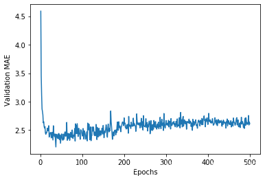
It may be a bit hard to see the plot due to scaling issues and relatively high variance. Let’s:
- Omit the first 10 data points, which are on a different scale from the rest of the curve.
- Replace each point with an exponential moving average of the previous points, to obtain a smooth curve.
因为纵轴的范围较大,且数据方差相对较大,所以难以看清这张图的规律。我们来重新绘制一张图。
‰ 删除前 10 个数据点,因为它们的取值范围与曲线上的其他点不同。
‰ 将每个数据点替换为前面数据点的指数移动平均值,以得到光滑的曲线。
def smooth_curve(points, factor=0.9):
  smoothed_points = []
  for point in points:
    if smoothed_points:
      previous = smoothed_points[-1]
      smoothed_points.append(previous * factor + point * (1 - factor))
    else:
      smoothed_points.append(point)
  return smoothed_points

smooth_mae_history = smooth_curve(average_mae_history[10:])

plt.plot(range(1, len(smooth_mae_history) + 1), smooth_mae_history)
plt.xlabel('Epochs')
plt.ylabel('Validation MAE')
plt.show()
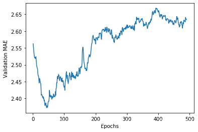
According to this plot, it seems that validation MAE stops improving significantly after 80 epochs. Past that point, we start overfitting.
Once we are done tuning other parameters of our model (besides the number of epochs, we could also adjust the size of the hidden layers), we
can train a final “production” model on all of the training data, with the best parameters, then look at its performance on the test data:
从图 3-13 可以看出,验证 MAE 在 80 轮后不再显著降低,之后就开始过拟合。
完成模型调参之后(除了轮数,还可以调节隐藏层大小),你可以使用最佳参数在所有训练数据上训练最终的生产模型,然后观察模型在测试集上的性能。
# Get a fresh, compiled model.
model = build_model()
# Train it on the entirety of the data.
model.fit(train_data, train_targets,
          epochs=80, batch_size=16, verbose=0)
test_mse_score, test_mae_score = model.evaluate(test_data, test_targets)
102/102 [==============================] - 0s 244us/step
test_mae_score
2.76008677482605
We are still off by about $2,550.
Wrapping up
Here’s what you should take away from this example:
- Regression is done using different loss functions from classification; Mean Squared Error (MSE) is a commonly used loss function for
regression. - Similarly, evaluation metrics to be used for regression differ from those used for classification; naturally the concept of “accuracy”
does not apply for regression. A common regression metric is Mean Absolute Error (MAE). - When features in the input data have values in different ranges, each feature should be scaled independently as a preprocessing step.
- When there is little data available, using K-Fold validation is a great way to reliably evaluate a model.
- When little training data is available, it is preferable to use a small network with very few hidden layers (typically only one or two),
in order to avoid severe overfitting.
This example concludes our series of three introductory practical examples. You are now able to handle common types of problems with vector data input:
- Binary (2-class) classification.
- Multi-class, single-label classification.
- Scalar regression.
In the next chapter, you will acquire a more formal understanding of some of the concepts you have encountered in these first examples,
such as data preprocessing, model evaluation, and overfitting.
总结
下面是你应该从这个例子中学到的要点。
‰ 回归问题使用的损失函数与分类问题不同。回归常用的损失函数是均方误差(MSE)。
‰ 同样,回归问题使用的评估指标也与分类问题不同。显而易见,精度的概念不适用于回归问题。常见的回归指标是平均绝对误差(MAE)。
‰ 如果输入数据的特征具有不同的取值范围,应该先进行预处理,对每个特征单独进行缩放。
‰ 如果可用的数据很少,使用 K 折验证可以可靠地评估模型。
‰ 如果可用的训练数据很少,最好使用隐藏层较少(通常只有一到两个)的小型网络,以避免严重的过拟合。
现在你可以处理关于向量数据最常见的机器学习任务了:
‰ 二分类问题、
‰ 多分类问题和标
‰ 标量量回归问题。