前言
们这里要解决的问题是,将手写数字的灰度图像(28 像素×28 像素)划分到 10 个类别中(0~9)。我们将使用 MNIST 数据集,它是机器学习领域的一个经典数据集,其历史几乎和这个领域一样长,而且已被人们深入研究。这个数据集包含 60 000 张训练图像和 10 000 张测试图像,由美国国家标准与技术研究院(National Institute of Standards and Technology,即 MNIST 中
的 NIST)在 20 世纪 80 年代收集得到。你可以将“解决”MNIST 问题看作深度学习的“Hello
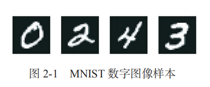
World”,正是用它来验证你的算法是否按预期运行。当你成为机器学习从业者后,会发现MNIST 一次又一次地出现在科学论文、博客文章等中。图 2-1 给出了 MNIST 数据集的一些样本。
关于类和标签的说明
在机器学习中,分类问题中的某个类别叫作类(class)。数据点叫作样本(sample)。某个样本对应的类叫作标签(label)。

代码
import keras
keras.__version__
Using TensorFlow backend.

'2.3.1'
A first look at a neural network
This notebook contains the code samples found in Chapter 2, Section 1 of Deep Learning with Python. Note that the original text features far more content, in particular further explanations and figures: in this notebook, you will only find source code and related comments.
We will now take a look at a first concrete example of a neural network, which makes use of the Python library Keras to learn to classify
hand-written digits. Unless you already have experience with Keras or similar libraries, you will not understand everything about this
first example right away. You probably haven’t even installed Keras yet. Don’t worry, that is perfectly fine. In the next chapter, we will
review each element in our example and explain them in detail. So don’t worry if some steps seem arbitrary or look like magic to you!
We’ve got to start somewhere.
The problem we are trying to solve here is to classify grayscale images of handwritten digits (28 pixels by 28 pixels), into their 10
categories (0 to 9). The dataset we will use is the MNIST dataset, a classic dataset in the machine learning community, which has been
around for almost as long as the field itself and has been very intensively studied. It’s a set of 60,000 training images, plus 10,000 test
images, assembled by the National Institute of Standards and Technology (the NIST in MNIST) in the 1980s. You can think of “solving” MNIST
as the “Hello World” of deep learning – it’s what you do to verify that your algorithms are working as expected. As you become a machine
learning practitioner, you will see MNIST come up over and over again, in scientific papers, blog posts, and so on.
初识神经网络
本笔记本包含在《Python深度学习》的第2章第1节中找到的代码示例。请注意,原始文本的内容更多,尤其是进一步的说明和附图:在本笔记本中,您将仅找到源代码和相关注释。
我们来看一个具体的神经网络示例,使用 Python 的 Keras 库来学习手写数字分类。如果你没用过 Keras 或类似的库,可能无法立刻搞懂这个例子中的全部内容。甚至你可能还没有安装Keras。没关系,下一章会详细解释这个例子中的每个步骤。因此,如果其中某些步骤看起来有
些随意,或者像魔法一样,也请你不要担心。下面我们要开始了。
我们这里要解决的问题是,将手写数字的灰度图像(28 像素×28 像素)划分到 10 个类别中(0~9)。我们将使用 MNIST 数据集,它是机器学习领域的一个经典数据集,其历史几乎和这个领域一样长,而且已被人们深入研究。这个数据集包含 60 000 张训练图像和 10 000 张测试像,由美国国家标准与技术研究院(National Institute of Standards and Technology,即 MNIST 中的 NIST)在 20 世纪 80 年代收集得到。你可以将“解决”MNIST 问题看作深度学习的“Hello World”,正是用它来验证你的算法是否按预期运行。当你成为机器学习从业者后,会发现MNIST 一次又一次地出现在科学论文、博客文章等中。
The MNIST dataset comes pre-loaded in Keras, in the form of a set of four Numpy arrays:
MNIST 数据集预先加载在 Keras 库中,其中包括 4 个 Numpy 数组。
from keras.datasets import mnist

(train_images, train_labels), (test_images, test_labels) = mnist.load_data()
# 国内可能有墙吧,下载不下来,我自己手动下载mnist.npz到本地,直接移到文件夹.kerasdatasets下
train_images and train_labels form the “training set”, the data that the model will learn from. The model will then be tested on the
“test set”, test_images and test_labels. Our images are encoded as Numpy arrays, and the labels are simply an array of digits, ranging
from 0 to 9. There is a one-to-one correspondence between the images and the labels.
Let’s have a look at the training data:
train_images 和 train_labels 组成了训练集(training set),模型将从这些数据中进行学习。然后在测试集(test set,即 test_images 和 test_labels)上对模型进行测试。图像被编码为 Numpy 数组,而标签是数字数组,取值范围为 0~9。图像和标签一一对应。
我们来看一下训练数据:
train_images.shape
(60000, 28, 28)
len(train_labels)
60000
train_labels
array([5, 0, 4, ..., 5, 6, 8], dtype=uint8)
Let’s have a look at the test data:
下面是测试数据:
test_images.shape
(10000, 28, 28)
len(test_labels)
10000
test_labels
array([7, 2, 1, ..., 4, 5, 6], dtype=uint8)
Our workflow will be as follow: first we will present our neural network with the training data, train_images and train_labels. The
network will then learn to associate images and labels. Finally, we will ask the network to produce predictions for test_images, and we
will verify if these predictions match the labels from test_labels.
Let’s build our network – again, remember that you aren’t supposed to understand everything about this example just yet.
接下来的工作流程如下:首先,将训练数据(train_images 和 train_labels)输入神经网络;其次,网络学习将图像和标签关联在一起;最后,网络对 test_images 生成预测,
而我们将验证这些预测与 test_labels 中的标签是否匹配。
下面我们来构建网络。再说一遍,你现在不需要理解这个例子的全部内容。
from keras import models
from keras import layers

network = models.Sequential()
network.add(layers.Dense(512, activation='relu', input_shape=(28 * 28,)))
network.add(layers.Dense(10, activation='softmax'))
The core building block of neural networks is the “layer”, a data-processing module which you can conceive as a “filter” for data. Some
data comes in, and comes out in a more useful form. Precisely, layers extract representations out of the data fed into them – hopefully
representations that are more meaningful for the problem at hand. Most of deep learning really consists of chaining together simple layers
which will implement a form of progressive “data distillation”. A deep learning model is like a sieve for data processing, made of a
succession of increasingly refined data filters – the “layers”.
Here our network consists of a sequence of two Dense layers, which are densely-connected (also called “fully-connected”) neural layers.
The second (and last) layer is a 10-way “softmax” layer, which means it will return an array of 10 probability scores (summing to 1). Each
score will be the probability that the current digit image belongs to one of our 10 digit classes.
To make our network ready for training, we need to pick three more things, as part of “compilation” step:
- A loss function: the is how the network will be able to measure how good a job it is doing on its training data, and thus how it will be
able to steer itself in the right direction. - An optimizer: this is the mechanism through which the network will update itself based on the data it sees and its loss function.
- Metrics to monitor during training and testing. Here we will only care about accuracy (the fraction of the images that were correctly
classified).
The exact purpose of the loss function and the optimizer will be made clear throughout the next two chapters.
神经网络的核心组件是层(layer),它是一种数据处理模块,你可以将它看成数据过滤器。进去一些数据,出来的数据变得更加有用。具体来说,层从输入数据中提取表示——我们期望
这种表示有助于解决手头的问题。大多数深度学习都是将简单的层链接起来,从而实现渐进式的数据蒸馏(data distillation)。深度学习模型就像是数据处理的筛子,包含一系列越来越精细的
数据过滤器(即层)。
本例中的网络包含 2 个 Dense 层,它们是密集连接(也叫全连接)的神经层。第二层(也是最后一层)是一个 10 路 softmax 层,它将返回一个由 10 个概率值(总和为 1)组成的数组。
每个概率值表示当前数字图像属于 10 个数字类别中某一个的概率要想训练网络,我们还需要选择编译(compile)步骤的三个参数。
‰ 损失函数(loss function):网络如何衡量在训练数据上的性能,即网络如何朝着正确的
方向前进。
‰ 优化器(optimizer):基于训练数据和损失函数来更新网络的机制。
‰ 在训练和测试过程中需要监控的指标(metric):本例只关心精度,即正确分类的图像所占的比例。
后续两章会详细解释损失函数和优化器的确切用途。
network.compile(optimizer='rmsprop',
                loss='categorical_crossentropy',
                metrics=['accuracy'])
Before training, we will preprocess our data by reshaping it into the shape that the network expects, and scaling it so that all values are in
the [0, 1] interval. Previously, our training images for instance were stored in an array of shape (60000, 28, 28) of type uint8 with
values in the [0, 255] interval. We transform it into a float32 array of shape (60000, 28 * 28) with values between 0 and 1.
在开始训练之前,我们将对数据进行预处理,将其变换为网络要求的形状,并缩放到所有值都在 [0, 1] 区间。比如,之前训练图像保存在一个 uint8 类型的数组中,其形状为
(60000, 28, 28),取值区间为 [0, 255]。我们需要将其变换为一个 float32 数组,其形状为 (60000, 28 * 28),取值范围为 0~1。
train_images = train_images.reshape((60000, 28 * 28))
train_images = train_images.astype('float32') / 255

test_images = test_images.reshape((10000, 28 * 28))
test_images = test_images.astype('float32') / 255
We also need to categorically encode the labels, a step which we explain in chapter 3:
我们还需要对标签进行分类编码,第 3 章将会对这一步骤进行解释。
from keras.utils import to_categorical

train_labels = to_categorical(train_labels)
test_labels = to_categorical(test_labels)
We are now ready to train our network, which in Keras is done via a call to the fit method of the network:
we “fit” the model to its training data.
现在我们准备开始训练网络,在 Keras 中这一步是通过调用网络的 fit 方法来完成的——我们在训练数据上拟合(fit)模型。
network.fit(train_images, train_labels, epochs=5, batch_size=128)
Epoch 1/5
60000/60000 [==============================] - 6s 93us/step - loss: 0.2571 - accuracy: 0.9251
Epoch 2/5
60000/60000 [==============================] - 2s 35us/step - loss: 0.1034 - accuracy: 0.9694
Epoch 3/5
60000/60000 [==============================] - 2s 29us/step - loss: 0.0685 - accuracy: 0.9791
Epoch 4/5
60000/60000 [==============================] - 2s 29us/step - loss: 0.0492 - accuracy: 0.9855
Epoch 5/5
60000/60000 [==============================] - 2s 29us/step - loss: 0.0373 - accuracy: 0.9893


<keras.callbacks.callbacks.History at 0x2041dbe0f88>
Two quantities are being displayed during training: the “loss” of the network over the training data, and the accuracy of the network over
the training data.
We quickly reach an accuracy of 0.989 (i.e. 98.9%) on the training data. Now let’s check that our model performs well on the test set too:
训练过程中显示了两个数字:一个是网络在训练数据上的损失(loss),另一个是网络在训练数据上的精度(acc)。
我们很快就在训练数据上达到了 0.989(98.9%)的精度。现在我们来检查一下模型在测试
集上的性能。
test_loss, test_acc = network.evaluate(test_images, test_labels)
10000/10000 [==============================] - 1s 66us/step
print('test_acc:', test_acc)
test_acc: 0.9797000288963318
Our test set accuracy turns out to be 97.8% – that’s quite a bit lower than the training set accuracy.
This gap between training accuracy and test accuracy is an example of “overfitting”,
the fact that machine learning models tend to perform worse on new data than on their training data.
Overfitting will be a central topic in chapter 3.
This concludes our very first example – you just saw how we could build and a train a neural network to classify handwritten digits, in
less than 20 lines of Python code. In the next chapter, we will go in detail over every moving piece we just previewed, and clarify what is really
going on behind the scenes. You will learn about “tensors”, the data-storing objects going into the network, about tensor operations, which
layers are made of, and about gradient descent, which allows our network to learn from its training examples.
测试集精度为 97.8%,比训练集精度低不少。训练精度和测试精度之间的这种差距是过拟合(overfit)造成的。过拟合是指机器学习模型在新数据上的性能往往比在训练数据上要差,它
是第 3 章的核心主题。
第一个例子到这里就结束了。你刚刚看到了如何构建和训练一个神经网络,用不到 20 行的Python 代码对手写数字进行分类。下一章会详细介绍这个例子中的每一个步骤,并讲解其背后
的原理。接下来你将要学到张量(输入网络的数据存储对象)、张量运算(层的组成要素)和梯度下降(可以让网络从训练样本中进行学习)。