支持向量机

支持向量机

一．基础知识:

• 概念及定义:
  支持向量机是一个二类分类模型，基本模型的定义为：是在特征空间上的间隔最大的线性分类器
  支持向量机学习的基本想法是求解能够正确划分训练数据集并且几何间隔最大的分离超平面．
  

• 二次规划是一类典型的优化问题,包括凸二次优化和非凸二次优化
  目标函数是变量的二次函数,约束条件是变量的线性不等式

• 核技巧(kernel trick):
  一般用来解决非线性分类问题,将非线性问题转换成线性问题
  第一步:首先使用一个变换将原空间的数据映射到新空间
  第二步:在新的空间里用线性分类学习方法从训练数据中学习分类模型

• 专有概念及名词
  1.函数间隔(functional margin):用 (hat{gamma}=y(wcdot x+b)) 来表示分类的正确性及确信度．
  2.几何间隔(geometric margin):对分离超平面进行规范化，例如(left|w ight|=1),这个时候函数间隔成为几何间隔．
  3.样本点((x_{i},y_{i}))和超平面((w,b))的几何间隔$$ gamma_{i}=y_{i}(frac{w}{left|w ight|}cdot x_{i}+frac{b}{left|w ight|}) $$ 取集合中所有样本点中几何间隔最小值$$gamma=min_{i=1,...N}gamma_{i}$$
  4.软间隔最大化：对于线性不可分的问题，通过修改约束条件实现数据的近似线性可分．叫做线性支持向量机的软间隔最大化
  5.支持向量机不仅可以用于分类问题，在回归问题上也可以较好的使用．

• 支持向量回归(support vector regression)SVR:
  支持向量回归有一个容忍偏差范围，当预计值和结果的偏差在范围（相当于间隔的一个区间）之内则认为预测是正确的．

二．思想脉络

• 所有的机器学习方法：
  

[方法＝策略＋模型＋算法$$<br>1.模型：就是假设空间的公式(条件概率分布和决策函数)<br>2.策略：选择最优的模型(利用损失函数，风险函数来进行选择)<br>3.算法：具体的计算方法(求解最优模型) - **支持向量机**的学习目标：<br>在特征空间中找到一个分离超平面，能够将实例分到不同的类，分离超平面对应于方程$$wcdot x+b=0$$ 由法向量和截距决定，分离超平面将特征空间分成两类，一部分是正类，一部分是负类．法向量指向的一侧为正类，另一侧为负类．<br>利用间隔最大化来寻找分离超平面 - **间隔最大化**:<br>求解间隔最大分离超平面，可表示为下面的约束最优化问题：$$max_{w,b} gamma$$ $$ s.t. y_{i}(frac{w}{left|w ight|}cdot x_{i}+frac{b}{left|w ight|})geq gamma, i=1,2...N 　　公式１$$<br>考虑到函数间隔和几何间隔之间的关系，可将问题改写成$$max_{w,b} frac{hat{gamma}}{left|w ight|}$$ $$ s.t. y_{i}(wcdot x_{i}+b)geq hat{gamma}, i=1,2...N 　　公式２$$<br>函数间隔的取值不影响函数最优化问题的解．取$hat{gamma}=1$注意到最大化$frac{1}{left|w ight|}$和最小化$frac{1}{2}left|w ight|^{2}$ 是等价的．<br>得到线性可分支持向量机的学习最优化问题：$$min_{w,b} frac{1}{2}left|w ight|^{2} $$ $$ s.t. y_{i}(wcdot x_{i}+b)-1geq 0, i=1,2...N　　公式３]

• 凸最优化问题:
  凸最优化问题变成凸二次规划问题(convex quadratic programming)
  根据上述公式３求得最优解　(w^{*},b^{*})得到分离超平面(w^{*}cdot x+b^{*}=0)
  分类决策函数$$f(x)=sign(w^{}cdot x+b^{})$$

2018.06.22　继续学习

• 线性不可分与软间隔最大化:
  主要操作就是将函数间隔大于等于１的条件进行放松．有些点可以出现在＂间隔＂里
  学习问题变成：$$min_{w,b,xi} frac{1}{2}left|w ight|^{{2}+Csum_{i=1}}{N}xi_{i}$$ $$s.t. y_{i}(wcdot x_{i}+b)geq 1-xi_{i},i=1,2,...,N$$ $$xi_{i}geq 0 ,i=1,2,...,N $$

• 线性不可分与核技巧:
  核技巧，用线性分类方法求解非线性分类问题：
  第一步：利用一个变换，将原数据的空间映射到新空间
  第二步：在新空间里用线性分类学习方法从训练数据集中学习分类模型
  最重要的就是核函数的选择，＂核函数选择＂就是意味着将样本映射到一个指定的特征空间，特征空间对于支持向量机的好坏影响很大．也就是划分的选择．

三．算法推导

• 对偶问题求解
  备注：拉格朗日对偶性 参考李航<统计学习方法>附录C.
  拉格朗日对偶：https://www.cnblogs.com/ooon/p/5723725.html

• dual problem:
  1.对每条约束添加拉格朗日乘子(alpha_{i}geq 0),拉格朗日函数可以写成$$L(w,x,alpha)=frac{1}{2}left|w ight|^{{2}+sum_{i=1}}{m} alpha_{i}(1-y_{i}(w^{T}x_{i}+b)) $$ 其中(alpha=(alpha_{1};alpha_{2};...alpha_{m})).
  (L(w,b,a)对w,b分别进行求偏导，令其值为０)可得:$$w=sum_{i=1}^{m}alpha_{i}y_{i}w_{i}$$ $$0=sum_{i=1}^{m}alpha_{i}y_{i}$$
  有上述公式及定义可得$$f(x)=frac{1}{2}left|w ight|^{2}=max_{w,b}L(w,b,alpha)$$

• 原始问题：
  $$min_{x}　f(x)$$ $$s.t. h_{i}(x)leq 0$$

• 对偶问题：
  推导对偶问题
  
  1.常通过将拉格朗日乘子对(w,b)求导并令其导数为0，来得到对偶函数的表达式
  
  2.对偶函数给出了主问题(原始问题)最优值的下界
  
  转变成对偶问题后，(L(w,b,alpha))是一个二次函数，可以求导求解其极小值．然后继续求解其中的极大值．

• 运算过程:
  1.求解(min_{w,b} L(w,b,alpha))
  2.二次函数求极值问题$$frac{mathrm{d} L(w,b,alpha)}{mathrm{d} w }=w-sum_{i=1}^{N} alpha_{i}y_{i}x_{i}=0$$ $$frac{mathrm{d} L(w,b,alpha)}{mathrm{d} b }=-sum_{i=1}^{N} alpha_{i}y_{i}=0$$
  求解后得：$$w=sum_{i=1}^{N} alpha_{i}y_{i}x_{i}$$

[0=sum_{i=1}^{N} alpha_{i}y_{i}$$ <br>将上述解代入到公式$L(w,b,a)$中： $$L(w,b,a)=frac{1}{2} sum_{i=1}^{N} sum_{j=1}^{N}alpha_{i}alpha_{j}y_{i}y_{j}(x_{i}cdot x_{j})-sum_{i}^{N}alpha_{i}y{i}left [ (sum_{j=1}^{N}alpha_{j}y_{j}x_{j})cdot x_{i} +b ight ]+sum_{i=1}^{N}alpha_{i}]

[=-frac{1}{2} sum_{i=1}^{N} sum_{j=1}^{N}alpha_{i}alpha_{j}y_{i}y_{j}(x_{i}cdot x_{j})+sum_{i=1}^{N}alpha_{i}$$<br>故可得：$$min_{w.b} L(w,b,alpha)=-frac{1}{2} sum_{i=1}^{N} sum_{j=1}^{N}alpha_{i}alpha_{j}y_{i}y_{j}(x_{i}cdot x_{j})+sum_{i=1}^{N}alpha_{i}$$<br>3.求解$min_{w,b}L(w,b,alpha)$的极大值 $$max_{alpha}-frac{1}{2} sum_{i=1}^{N} sum_{j=1}^{N}alpha_{i}alpha_{j}y_{i}y_{j}(x_{i}cdot x_{j})+sum_{i=1}^{N}alpha_{i}]

[s.t. sum_{i=1}^{N}alpha_{i}y_{i}=0$$ $$ alpha_{i} geq 0 ,i=1,2,...,N $$ <br>可转换成$$min_{alpha} frac{1}{2} sum_{i=1}^{N} sum_{j=1}^{N}alpha_{i}alpha_{j}y_{i}y_{j}(x_{i}cdot x_{j})-sum_{i=1}^{N}alpha_{i} ]

[s.t. sum_{i=1}^{N}alpha_{i}y_{i}=0$$ $$ alpha_{i} geq 0 ,i=1,2,...,N $$ <br>4.根据定理进行求解$w^{*},b^{*}$: $$w^{*}=sum_{i=1}^{N}alpha_{i}^{*}y_{j}x_{j}]

[b^{*}=y_{j}-sum_{i=1}^{N}alpha_{i}^{*}y_{i}(x_{i}cdot x_{j}) ]

• 分离超平面:
  

[sum_{i=1}^{N}alpha_{i}^{*}y_{i}(x_{i}cdot x_{j})+b^{*}=0 ]

• 分类决策函数:
  

[f(x)=signleft (sum_{i=1}^{N}alpha_{i}^{*}y_{i}(x_{i}cdot x_{j})+b^{*} ight )$$<br>对于软间隔最大化，求解的思路是一样的，不同点就是构造的拉格朗日函数不同以及约束条件不同<br>核函数的相关求解，理论方面还是没有理解透彻．还需要继续学习 <font color=red size=2> 学习断点　核函数理论的理解　</font> [关于公式理论及SMO更详细的推导](https://app.yinxiang.com/shard/s56/nl/20932638/cf719393-2c0f-4c15-870c-96d488f649dc/) ###四．编程实现 - 2.序列最小最优化算法 - **sequential minimal optimization SMO算法**：<br>核函数的理解:将一个欧式空间映射到希尔伯特空间的一个函数<br> 核函数的选择是支持向量机的最大变数,核函数的选取一般也是按照经验公式来进行选取<br>例如:文本数据通常采用线性核,情况不明确的时候可以尝试高斯核 - 3.利用线性核&高斯核训练一个SVM,并比较支持向量的区别 - 3.1数据的读取和可视化处理 ```python # 西瓜数据集的读取 import pandas as pd with open('/home/dengshuo/GithubCode/ML/CH06/watermelon_3a.csv') as datafile: df=pd.read_csv(datafile ,header=None) print (df) ``` - - 0 1 2 3 0 1 0.697 0.4600 1 1 2 0.774 0.3760 1 2 3 0.634 0.2640 1 3 4 0.608 0.3180 1 4 5 0.556 0.2150 1 5 6 0.403 0.2370 1 6 7 0.481 0.1490 1 7 8 0.437 0.2110 1 8 9 0.666 0.0910 0 9 10 0.243 0.0267 0 10 11 0.245 0.0570 0 11 12 0.343 0.0990 0 12 13 0.639 0.1610 0 13 14 0.657 0.1980 0 14 15 0.360 0.3700 0 15 16 0.593 0.0420 0 16 17 0.719 0.1030 0 read_csv() arg header: int or list of ints, default 'infer' Row number(s) to use as the column names, and the start of the data. Default behavior is as if set to 0 if no ``names`` passed, otherwise ``None``. Explicitly pass ``header=0`` to be able to replace existing names. The header can be a list of integers that specify row locations for a multi-index on the columns e.g. [0,1,3]. Intervening rows that are not specified will be skipped (e.g. 2 in this example is skipped). Note that this parameter ignores commented lines and empty lines if ``skip_blank_lines=True``, so header=0 denotes the first line of data rather than the first line of the file. ```python # 制作表头 : 将每列数据填上标签,将每列数据进行命名, # 当原始的数据中含有名字时,可以直接进行读取 # make header df.columns=['id','density','sugar_content','label'] print(df) ``` - id density sugar_content label 0 1 0.697 0.4600 1 1 2 0.774 0.3760 1 2 3 0.634 0.2640 1 3 4 0.608 0.3180 1 4 5 0.556 0.2150 1 5 6 0.403 0.2370 1 6 7 0.481 0.1490 1 7 8 0.437 0.2110 1 8 9 0.666 0.0910 0 9 10 0.243 0.0267 0 10 11 0.245 0.0570 0 11 12 0.343 0.0990 0 12 13 0.639 0.1610 0 13 14 0.657 0.1980 0 14 15 0.360 0.3700 0 15 16 0.593 0.0420 0 16 17 0.719 0.1030 0 ```python # 更改索引列 df.set_index 将原先按第一列的数据,按要求的列进行索引 df.set_index(['id']) ``` <div> <style> .dataframe thead tr:only-child th { text-align: right; } .dataframe thead th { text-align: left; } .dataframe tbody tr th { vertical-align: top; } </style> <table border="1" class="dataframe"> <thead> <tr style="text-align: right;"> <th></th> <th>density</th> <th>sugar_content</th> <th>label</th> </tr> <tr> <th>id</th> <th></th> <th></th> <th></th> </tr> </thead> <tbody> <tr> <th>1</th> <td>0.697</td> <td>0.4600</td> <td>1</td> </tr> <tr> <th>2</th> <td>0.774</td> <td>0.3760</td> <td>1</td> </tr> <tr> <th>3</th> <td>0.634</td> <td>0.2640</td> <td>1</td> </tr> <tr> <th>4</th> <td>0.608</td> <td>0.3180</td> <td>1</td> </tr> <tr> <th>5</th> <td>0.556</td> <td>0.2150</td> <td>1</td> </tr> <tr> <th>6</th> <td>0.403</td> <td>0.2370</td> <td>1</td> </tr> <tr> <th>7</th> <td>0.481</td> <td>0.1490</td> <td>1</td> </tr> <tr> <th>8</th> <td>0.437</td> <td>0.2110</td> <td>1</td> </tr> <tr> <th>9</th> <td>0.666</td> <td>0.0910</td> <td>0</td> </tr> <tr> <th>10</th> <td>0.243</td> <td>0.0267</td> <td>0</td> </tr> <tr> <th>11</th> <td>0.245</td> <td>0.0570</td> <td>0</td> </tr> <tr> <th>12</th> <td>0.343</td> <td>0.0990</td> <td>0</td> </tr> <tr> <th>13</th> <td>0.639</td> <td>0.1610</td> <td>0</td> </tr> <tr> <th>14</th> <td>0.657</td> <td>0.1980</td> <td>0</td> </tr> <tr> <th>15</th> <td>0.360</td> <td>0.3700</td> <td>0</td> </tr> <tr> <th>16</th> <td>0.593</td> <td>0.0420</td> <td>0</td> </tr> <tr> <th>17</th> <td>0.719</td> <td>0.1030</td> <td>0</td> </tr> </tbody> </table> </div> ```python # 数据进行可视化处理 import numpy as np import matplotlib.pyplot as plt import seaborn as sns fig=plt.figure() ax=fig.add_subplot(111) ax.scatter(df['density'],df['sugar_content']) plt.show() ```  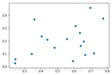可以画出一个最基本的图形,但是这个只能反映出两个变量之间的函数关系 没有显示出好坏瓜与两个变量之间的联系.label 没有表现出来 ```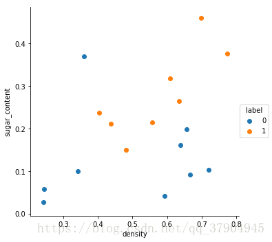python # 利用matplotlib & seaborn 来进行画图 plt.figure(0) sns.FacetGrid(df,hue='label',size=5).map(plt.scatter,'density','sugar_content').add_legend() plt.show() ``` <matplotlib.figure.Figure at 0x7f671a0a9d30>  ```python df[['density','sugar_content']].values ``` - - array([[ 0.697 , 0.46 ], [ 0.774 , 0.376 ], [ 0.634 , 0.264 ], [ 0.608 , 0.318 ], [ 0.556 , 0.215 ], [ 0.403 , 0.237 ], [ 0.481 , 0.149 ], [ 0.437 , 0.211 ], [ 0.666 , 0.091 ], [ 0.243 , 0.0267], [ 0.245 , 0.057 ], [ 0.343 , 0.099 ], [ 0.639 , 0.161 ], [ 0.657 , 0.198 ], [ 0.36 , 0.37 ], [ 0.593 , 0.042 ], [ 0.719 , 0.103 ]]) - 利用seaborn可以表示三个维度 row ,columns,hue hue 利用颜色的不同来进行区分 - 3.2 调用机器学习包来实现算法<br>下面是一个最简单的基本流程,可以用来模仿<br> help(plt.scatter) scatter(x, y, s=None, c=None, marker=None, cmap=None, norm=None, vmin=None, vmax=None, alpha=None, linewidths=None, verts=None, edgecolors=None, hold=None, data=None, **kwargs) help(plt.pcolorsmesh) pcolormesh(*args, **kwargs) Plot a quadrilateral mesh. 绘制一个四边形网格 help(np.meshgrid) meshgrid(*xi, **kwargs) Return coordinate matrices from coordinate vectors. 从坐标向量返回坐标矩阵 Make N-D coordinate arrays for vectorized evaluations of N-D scalar/vector fields over N-D grids, given one-dimensional coordinate arrays x1, x2,..., xn. 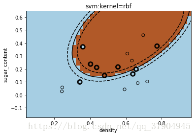```python # import library from sklearn import svm # assumed you have X (predictor) and Y(target) #Create SVM classification object model=svm.SVC(C=1000,kernel='rbf') # Penalty parameter C of the error term. # 这个C 是个错误项的惩罚参数 # 可直接通过改变核函数来进行 #　或者定义一个循环来进行 # for fig_num ,kernel in enumerate(('linear','rbf')): # model=svm.SVC(C=1000,kernel=kernel) # 涉及的变量进行修改 # train the model using the training sets and check score X=df[['density','sugar_content']].values y=df['label'].values model.fit(X,y) # get support vectors sv=model.support_vectors_ # draw decision zone plt.figure('rbf') plt.clf() # plot point and mark out support vectors plt.scatter(X[:,0],X[:,1],edgecolors='k',c=y,cmap=plt.cm.Paired,zorder=10) # 只有这一个 zorder 参数没有看懂,不是很明白是什么意思 plt.scatter(sv[:,0],sv[:,1],edgecolors='k',facecolors='none',s=80,linewidths=2,zorder=10) # plot the decision boundary and decision zone into a color plot x_min,x_max=X[:,0].min()-0.2 ,X[:,0].max()+0.2 y_min,y_max=X[:,1].min()-0.2 ,X[:,1].max()+0.2 XX,YY=np.meshgrid(np.arange(x_min,x_max,0.02),np.arange(y_min,y_max,0.02)) Z=model.decision_function(np.c_[XX.ravel(),YY.ravel()]) # decision_function(X) method of sklearn.svm.classes.SVC instance # Distance of the samples X to the separating hyperplane. 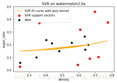Z=Z.reshape(XX.shape) plt.pcolormesh(XX,YY,Z>0,cmap=plt.cm.Paired) plt.contour(XX,YY,Z,colors=['k','k','k'],linestyles=['--','-','--'],levels=[-.5,0,.5]) plt.title('svm:kernel=rbf') plt.axis('tight') plt.xlabel('density') plt.ylabel('sugar_content') plt.show() ```  ####4. 利用西瓜数据集3.0a ,密度"density"为输入,含糖率"sugar_content"为输出.训练一个SVR ```python df.columns=['id','density','sugar_content','label'] df.set_index(['id']) ``` <div> <style> .dataframe thead tr:only-child th { text-align: right; } .dataframe thead th { text-align: left; } .dataframe tbody tr th { vertical-align: top; } </style> <table border="1" class="dataframe"> <thead> <tr style="text-align: right;"> <th></th> <th>density</th> <th>sugar_content</th> <th>label</th> </tr> <tr> <th>id</th> <th></th> <th></th> <th></th> </tr> </thead> <tbody> <tr> <th>1</th> <td>0.697</td> <td>0.4600</td> <td>1</td> </tr> <tr> <th>2</th> <td>0.774</td> <td>0.3760</td> <td>1</td> </tr> <tr> <th>3</th> <td>0.634</td> <td>0.2640</td> <td>1</td> </tr> <tr> <th>4</th> <td>0.608</td> <td>0.3180</td> <td>1</td> </tr> <tr> <th>5</th> <td>0.556</td> <td>0.2150</td> <td>1</td> </tr> <tr> <th>6</th> <td>0.403</td> <td>0.2370</td> <td>1</td> </tr> <tr> <th>7</th> <td>0.481</td> <td>0.1490</td> <td>1</td> </tr> <tr> <th>8</th> <td>0.437</td> <td>0.2110</td> <td>1</td> </tr> <tr> <th>9</th> <td>0.666</td> <td>0.0910</td> <td>0</td> </tr> <tr> <th>10</th> <td>0.243</td> <td>0.0267</td> <td>0</td> </tr> <tr> <th>11</th> <td>0.245</td> <td>0.0570</td> <td>0</td> </tr> <tr> <th>12</th> <td>0.343</td> <td>0.0990</td> <td>0</td> </tr> <tr> <th>13</th> <td>0.639</td> <td>0.1610</td> <td>0</td> </tr> <tr> <th>14</th> <td>0.657</td> <td>0.1980</td> <td>0</td> </tr> <tr> <th>15</th> <td>0.360</td> <td>0.3700</td> <td>0</td> </tr> <tr> <th>16</th> <td>0.593</td> <td>0.0420</td> <td>0</td> </tr> <tr> <th>17</th> <td>0.719</td> <td>0.1030</td> <td>0</td> </tr> </tbody> </table> </div> ```python X=df['density'] y=df['sugar_content'] plt.figure() plt.scatter(X,y,c='g') plt.xlabel('density') plt.ylabel('sugar_content') plt.show() # 但是这个图 没办法显示 好坏 瓜的关系 应该还有其他的办法 ```  ```python # 试着调用机器学习包 from sklearn import svm svr=svm.SVR() X=df['density'].values y=df['sugar_content'].values svr.fit(X,y) ``` ```python import pandas as pd import numpy as np import matplotlib.pyplot as plt from sklearn.svm import SVR # for SVR model from sklearn.model_selection import GridSearchCV # for optimal parameter search # loading data df = pd.read_csv('/home/dengshuo/GithubCode/ML/CH06/watermelon_3a.csv', header=None, ) df.columns = ['id', 'density', 'sugar_content', 'label'] df.set_index(['id']) X = df[['density']].values y = df[['sugar_content']].values # generate model and fitting # linear # svr = GridSearchCV(SVR(kernel='linear'), cv=5, param_grid={"C": [1e0, 1e1, 1e2, 1e3]}) # rbf # svr = GridSearchCV(SVR(kernel='rbf'), cv=5, param_grid={"C": [1e-4, 1e-3, 1e-2, 1e-1, 1, 1e1, 1e2, 1e3, 1e4]}) # ploy svr = GridSearchCV(SVR(kernel='poly'), cv=5, param_grid={"C": [1e-4, 1e-3, 1e-2, 1e-1, 1, 1e1, 1e2, 1e3, 1e4]}) svr.fit(X, y) sv_ratio = svr.best_estimator_.support_.shape[0] / len(X) print("Support vector ratio: %.3f" % sv_ratio) y_svr = svr.predict(X) sv_ind = svr.best_estimator_.support_ plt.scatter(X[sv_ind], y[sv_ind], c='r', s=50, label='SVR support vectors', zorder=2) plt.scatter(X, y, c='k', label='data', zorder=1) plt.plot(X, y_svr, c='orange', label='SVR fit curve with poly kernel') plt.xlabel('density') plt.ylabel('sugar_ratio') plt.title('SVR on watermelon3.0a') plt.legend() plt.show() ``` /home/dengshuo/anaconda3/lib/python3.6/site-packages/sklearn/utils/validation.py:578: DataConversionWarning: A column-vector y was passed when a 1d array was expected. Please change the shape of y to (n_samples, ), for example using ravel(). y = column_or_1d(y, warn=True) <br> - Support vector ratio: 0.471]