OSL回归
简单的线性回归
> fit<-lm(weight~height,women)
> summary(fit)

Call:
lm(formula = weight ~ height, data = women)

Residuals:
Min 1Q Median 3Q Max
-1.7333 -1.1333 -0.3833 0.7417 3.1167

Coefficients:
Estimate Std. Error t value Pr(>|t|)
(Intercept) -87.51667 5.93694 -14.74 1.71e-09 ***
height 3.45000 0.09114 37.85 1.09e-14 ***
---
Signif. codes: 0 ‘***’ 0.001 ‘**’ 0.01 ‘*’ 0.05 ‘.’ 0.1 ‘ ’ 1

Residual standard error: 1.525 on 13 degrees of freedom
Multiple R-squared: 0.991,	Adjusted R-squared: 0.9903
F-statistic: 1433 on 1 and 13 DF, p-value: 1.091e-14


> residuals(fit)
1 2 3 4 5
2.41666667 0.96666667 0.51666667 0.06666667 -0.38333333
6 7 8 9 10
-0.83333333 -1.28333333 -1.73333333 -1.18333333 -1.63333333
11 12 13 14 15
-1.08333333 -0.53333333 0.01666667 1.56666667 3.11666667


> fitted(fit)  #列出拟合模型的预测值
1 2 3 4 5 6 7 8 9
112.5833 116.0333 119.4833 122.9333 126.3833 129.8333 133.2833 136.7333 140.1833
10 11 12 13 14 15
143.6333 147.0833 150.5333 153.9833 157.4333 160.8833


> residuals(fit) #列出拟合模型的残差值
1 2 3 4 5 6 7
2.41666667 0.96666667 0.51666667 0.06666667 -0.38333333 -0.83333333 -1.28333333
8 9 10 11 12 13 14
-1.73333333 -1.18333333 -1.63333333 -1.08333333 -0.53333333 0.01666667 1.56666667
15
3.11666667


> plot(women$height~women$weight,xlab="Height (in inches)", ylab="Weight (in pounds)")
> abline(fit)
得到预测回归公式:Weight=-87.52+3.45*Height
多项式回归
fit2<-lm(weight~height+I(height^2), data=women)
> summary(fit2)

Call:
lm(formula = weight ~ height + I(height^2), data = women)

Residuals:
Min 1Q Median 3Q Max
-0.50941 -0.29611 -0.00941 0.28615 0.59706

Coefficients:
Estimate Std. Error t value Pr(>|t|)
(Intercept) 261.87818 25.19677 10.393 2.36e-07 ***
height -7.34832 0.77769 -9.449 6.58e-07 ***
I(height^2) 0.08306 0.00598 13.891 9.32e-09 ***
---
Signif. codes: 0 ‘***’ 0.001 ‘**’ 0.01 ‘*’ 0.05 ‘.’ 0.1 ‘ ’ 1

Residual standard error: 0.3841 on 12 degrees of freedom
Multiple R-squared: 0.9995,	Adjusted R-squared: 0.9994
F-statistic: 1.139e+04 on 2 and 12 DF, p-value: < 2.2e-16

> plot(women$height,women$weight,xlab="Height (in inches)",ylab="Weight (in lbs)")
> lines(women$height,fitted(fit2))

回归公式:Weight=261.88-7.35*Height+0.083*Height^2

三次方线性回归
fit3<-lm(weight~height+I(height^2)+I(height^3),data=women)

summary(fit3)

Call:
lm(formula = weight ~ height + I(height^2) + I(height^3), data = women)

Residuals:
Min 1Q Median 3Q Max
-0.40677 -0.17391 0.03091 0.12051 0.42191

Coefficients:
Estimate Std. Error t value Pr(>|t|)
(Intercept) -8.967e+02 2.946e+02 -3.044 0.01116 *
height 4.641e+01 1.366e+01 3.399 0.00594 **
I(height^2) -7.462e-01 2.105e-01 -3.544 0.00460 **
I(height^3) 4.253e-03 1.079e-03 3.940 0.00231 **
---
Signif. codes: 0 ‘***’ 0.001 ‘**’ 0.01 ‘*’ 0.05 ‘.’ 0.1 ‘ ’ 1

Residual standard error: 0.2583 on 11 degrees of freedom
Multiple R-squared: 0.9998,	Adjusted R-squared: 0.9997
F-statistic: 1.679e+04 on 3 and 11 DF, p-value: < 2.2e-16


plot(women$height,women$weight,xlab="height",ylab="weight")
lines(women$height,fitted(fit3))

回归公式:Weight=-8.967e+02 + 4.641e+01*Height -7.462e-01 * Height^2 + 4.253e-03 *Height^3

多元线性回归
fit<-lm(Murder~Population+Illiteracy+Income+Frost,data=states)
summary(fit)

Call:
lm(formula = Murder ~ Population + Illiteracy + Income + Frost,
data = states)

Residuals:
Min 1Q Median 3Q Max
-4.7960 -1.6495 -0.0811 1.4815 7.6210

Coefficients:
Estimate Std. Error t value Pr(>|t|)
(Intercept) 1.235e+00 3.866e+00 0.319 0.7510
Population 2.237e-04 9.052e-05 2.471 0.0173 *
Illiteracy 4.143e+00 8.744e-01 4.738 2.19e-05 ***
Income 6.442e-05 6.837e-04 0.094 0.9253
Frost 5.813e-04 1.005e-02 0.058 0.9541
---
Signif. codes: 0 ‘***’ 0.001 ‘**’ 0.01 ‘*’ 0.05 ‘.’ 0.1 ‘ ’ 1

Residual standard error: 2.535 on 45 degrees of freedom
Multiple R-squared: 0.567,	Adjusted R-squared: 0.5285
F-statistic: 14.73 on 4 and 45 DF, p-value: 9.133e-08
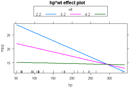
有交互项的多元线性回归
fit<-lm(mpg~hp+wt+hp:wt,data=mtcars)
summary(fit)

Call:
lm(formula = mpg ~ hp + wt + hp:wt, data = mtcars)

Residuals:
Min 1Q Median 3Q Max
-3.0632 -1.6491 -0.7362 1.4211 4.5513

Coefficients:
Estimate Std. Error t value Pr(>|t|)
(Intercept) 49.80842 3.60516 13.816 5.01e-14 ***
hp -0.12010 0.02470 -4.863 4.04e-05 ***
wt -8.21662 1.26971 -6.471 5.20e-07 ***
hp:wt 0.02785 0.00742 3.753 0.000811 ***
---
Signif. codes: 0 ‘***’ 0.001 ‘**’ 0.01 ‘*’ 0.05 ‘.’ 0.1 ‘ ’ 1

Residual standard error: 2.153 on 28 degrees of freedom
Multiple R-squared: 0.8848,	Adjusted R-squared: 0.8724
F-statistic: 71.66 on 3 and 28 DF, p-value: 2.981e-13


library(effects)
plot(effect("hp:wt",fit,,list(wt=c(2.2,3.2,4.2))),multiline=TRUE)
回归判断
fit<-lm(Murder~Population+Illiteracy+Income+Frost,data=states)
confint(fit)

                2.5 %                  97.5 %
(Intercept) -6.552191e+00     9.0213182149
Population 4.136397e-05      0.0004059867
Illiteracy 2.381799e+00        5.9038743192 #文盲改变1%,谋杀率就在改区间变动,它的置信区间为95%
Income -1.312611e-03         0.0014414600
Frost -1.966781e-02            0.0208304170


fit<-lm(weight~height,data=women)
par(mfrow=c(2,2))
plot(fit)


Residuals vs Fitted: 线性

Normal Q-Q: 正态性

Scale-Location:同方差性

fit2<-lm(weight~height+I(height^2),data=women)
par(nfrow=c(2,2))
plot(fit2)

newfit2<-lm(weight~height+I(height^2),data=women[-c(13,15),])  #排除异常点
par(nfrow=c(2,2))
plot(newfit2)

检测异常值
#离群点
library(car)
outlierTest(fit)

rstudent unadjusted p-value Bonferonni p
Nevada 3.542929 0.00095088 0.047544


#高杠杆值
hat.plot<-function(fit){
p<-length(coefficients(fit))
n<-length(fitted(fit))
plot(hatvalues(fit),main="Index Plot of Hat Values")
abline(h=c(2,3)*p/n,col="red",lty=2)
identify(1:n,hatvalues(fit),names(hatvalues(fit)))
}

hat.plot(fit)

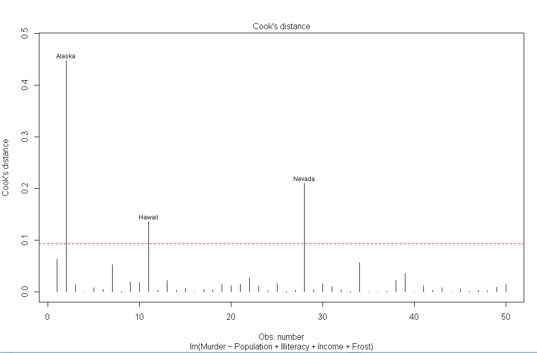
#强影响点
cutoff<-4/(nrow(states)-length(fit$coefficients)-2)
plot(fit,which=4,cook.levels=cutoff)
abline(h=cutoff,lty=2,col="red")
library(car)
avPlots(fit,ask=FALSE,id.method="identify")

library(car)
influencePlot(fit,id.method = "identify",main="Influence Plot",sub="Circle size is proportional to Cook's distance")

改进措施
#变量变换
library(car)
summary(powerTransform(states$Murder))

bcPower Transformation to Normality
Est Power Rounded Pwr Wald Lwr bnd Wald Upr Bnd
states$Murder 0.6055 1 0.0884 1.1227  #可以使用 0.6来正态化变量Murder, 例如 Murder ^ 0.6

Likelihood ratio tests about transformation parameters
LRT df pval
LR test, lambda = (0) 5.665991 1 0.01729694
LR test, lambda = (1) 2.122763 1 0.14512456
选择最佳回归模型
#排除不需要的随机变量
fit1<-lm(Murder~Population+Illiteracy+Income+Frost,data=states)
fit2<-lm(Murder~Population+Illiteracy,data=states)
anova(fit2,fit1)

AIC(fit1,fit2) #AIF 返回值越小,模型效果越佳,精简变量

df AIC
fit1 6 241.6429
fit2 4 237.6565


逐步回归

模型通过每次添加或删除一个变量来探索最佳的回归模型所需要的变量

library(MASS)
fit<-lm(Murder~Population+Illiteracy+Income+Frost,data=states)
stepAIC(fit,direction="backward")


Start: AIC=97.75
Murder ~ Population + Illiteracy + Income + Frost

Df Sum of Sq RSS AIC
- Frost 1 0.021 289.19 95.753
- Income 1 0.057 289.22 95.759
<none> 289.17 97.749
- Population 1 39.238 328.41 102.111
- Illiteracy 1 144.264 433.43 115.986

Step: AIC=95.75
Murder ~ Population + Illiteracy + Income

Df Sum of Sq RSS AIC
- Income 1 0.057 289.25 93.763
<none> 289.19 95.753
- Population 1 43.658 332.85 100.783
- Illiteracy 1 236.196 525.38 123.605

Step: AIC=93.76
Murder ~ Population + Illiteracy

Df Sum of Sq RSS AIC
<none> 289.25 93.763
- Population 1 48.517 337.76 99.516
- Illiteracy 1 299.646 588.89 127.311

Call:
lm(formula = Murder ~ Population + Illiteracy, data = states) 最佳模型公式

Coefficients:
(Intercept) Population Illiteracy
1.6515497 0.0002242 4.0807366


变量选择-全子集回归
install.packages("leaps")
library(leaps)
states<-as.data.frame(state.x77[,c("Murder","Population","Illiteracy","Income","Frost")])
leaps<-regsubsets(Murder~Population+Illiteracy+Income+Frost,data=states,nbest=4)
plot(leaps,scale="adjr2")

library(car)
subsets(leaps,statistic="cp",main="Cp Plot for All Subsets Regression")
abline(1,1,lty=2,col="red")  #离线越近,效果约好

#R平方的K重交叉验证
install.packages("bootstrap")
shrinkage<-function(fit,k=10)
{
require(bootstrap)
theta.fit<-function(x,y){lsfit(x,y)}
theta.predict<-function(fit,x){cbind(1,x)%*%fit$coef}

x<-fit$model[,2:ncol(fit$model)]
y<-fit$model[,1]

results<-crossval(x,y,theta.fit,theta.predict,ngroup=k)
r2<-cor(y,fit$fitted.values)^2
r2cv<-cor(y,results$cv.fit)^2
cat("Original R-square=",r2,"
")
cat(k,"Fold Cross-Validated R-square=",r2cv,"
")
cat("Change=",r2-r2cv,"
")

}
fit<-lm(Murder~Population+Illiteracy+Income+Frost,data=states)
shrinkage(fit)

Original R-square= 0.5669502
10 Fold Cross-Validated R-square= 0.4474345
Change= 0.1195158


fit2<-lm(Murder~Population+Illiteracy,data=states)
shrinkage(fit2)

Original R-square= 0.5668327
10 Fold Cross-Validated R-square= 0.5182764
Change= 0.0485563


相对重要性

检测模型中的变量重要性程度
zstates<-as.data.frame(scale(states))
zfit<-lm(Murder~Population+Income+Illiteracy+Frost,data=zstates)
coef(zfit)


(Intercept) Population Income Illiteracy Frost
-2.054026e-16 2.705095e-01 1.072372e-02 6.840496e-01 8.185407e-03 文盲率值最大,所以它在模型变量中的权重最大


变量权重


relweights <- function(fit,...){
R <- cor(fit$model)
nvar <- ncol(R)
rxx <- R[2:nvar, 2:nvar]
rxy <- R[2:nvar, 1]
svd <- eigen(rxx)
evec <- svd$vectors
ev <- svd$values
delta <- diag(sqrt(ev))
lambda <- evec %*% delta %*% t(evec)
lambdasq <- lambda ^ 2
beta <- solve(lambda) %*% rxy
rsquare <- colSums(beta ^ 2)
rawwgt <- lambdasq %*% beta ^ 2
import <- (rawwgt / rsquare) * 100
import <- as.data.frame(import)
row.names(import) <- names(fit$model[2:nvar])
names(import) <- "Weights"
import <- import[order(import),1, drop=FALSE]
dotchart(import$Weights, labels=row.names(import),
xlab="% of R-Square", pch=19,
main="Relative Importance of Predictor Variables",
sub=paste("Total R-Square=", round(rsquare, digits=3)),
...)
return(import)
}

fit<-lm(Murder~Population+Illiteracy+Income+Frost,data=states)
relweights(fit,col="blue")
