深度学习UFLDL老教程笔记1 稀疏自编码器Ⅱ

稀疏自编码器的学习结构:

稀疏自编码器Ⅰ：

神经网络

反向传导算法

梯度检验与高级优化

稀疏自编码器Ⅱ：

自编码算法与稀疏性

可视化自编码器训练结果

Exercise: Sparse Autoencoder

---

自编码算法与稀疏性

已经讨论了神经网络在有监督学习中的应用，其中训练样本是有类别标签的（x_i，y_i）。

自编码神经网络是一种无监督学习算法，它使用了反向传播算法，并让目标值等于输入值x_i = y_i 。

下图是一个自编码神经网络的示例。

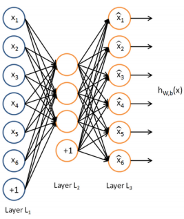
一次autoencoder学习，结构三层：输入层单元数=输出层单元数，隐藏层。自编码神经网络尝试学习一个输入约等于输出的恒等函数。

给自编码神经网络加入某些限制，我们就可以从输入数据中发现一些有趣的结构。比如限定隐藏神经元的数量。

隐藏层神经元的数量较小

比如使隐藏层神经元的数量<输入层神经元的数量<输出层经元的数量，迫使自编码神经网络去学习输入数据的压缩表示。

当输入数据是完全随机的，比如输入特征完全无关，难学习。

当输入数据中隐含着一些特定的结构，比如输入特征是彼此相关的，算法就可以发现输入数据中的这些相关性。

事实上，这一简单的自编码神经网络通常可以学习出一个跟主元分析（PCA）结果非常相似的输入数据的低维表示。

隐藏层神经元的数量较大

仍然通过给自编码神经网络施加一些其他的限制条件来发现输入数据中的结构。

给隐藏层神经元加入稀疏性限制

稀疏性可以被简单地解释如下。如果当神经元的输出接近于1的时候我们认为它被激活，而输出接近于0的时候认为它被抑制，那么使得神经元大部分的时间都是被抑制的限制则被称作稀疏性限制。这里我们假设的神经元的激活函数是sigmoid函数。如果你使用tanh作为激活函数的话，当神经元输出为-1的时候，我们认为神经元是被抑制的。

以上是稀疏性的含义，具体获得稀疏性的方法ufldl教程中有详细讲述，这里只说核心概念框架。

隐藏神经元 j的平均活跃度（在训练集上取平均）

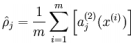
注意，计算用到了前向传播算法，而BP也用到了，内存够保存算一遍，否则两遍。

限制其中p是稀疏性参数，通常是一个接近于0的较小的值（比如 p=0.05 ）

为了实现这一限制，我们将会在我们的优化目标函数中加入一个额外的惩罚因子，而这一惩罚因子将惩罚那些 和 有显著不同的情况从而使得隐藏神经元的平均活跃度保持在较小范围内（稀疏性）。

惩罚因子的具体形式有很多种合理的选择，我们将会选择以下这一种：

    

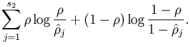
KL divergence 性质：相等为0，随着之间的差异增大而单调递增。

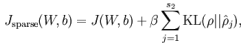
现在，我们的总体代价函数可以表示为：

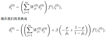
To incorporate the KL-divergence term into your derivative calculation, there is a simple-to-implement trick involving only a small change to your code.

具体地，在BP第二层中：

可视化自编码器训练结果

训练完（稀疏）自编码器，我们还想把这自编码器学到的函数可视化出来，好弄明白它到底学到了什么。我们以在10×10图像（即n=100）上训练自编码器为例。

Exercise: Sparse Autoencoder实验

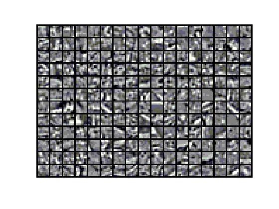
首先是从如下图这样的10 image（512×512），中sample 10000 image patches（8×8）。

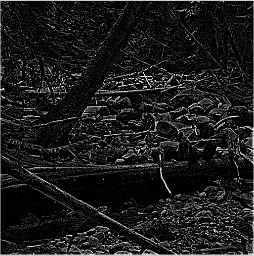
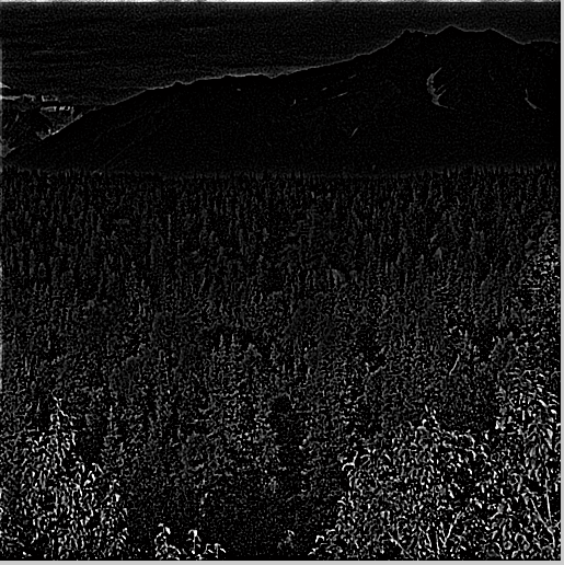
sample 10000 image patches（8×8） and concatenate them into a 64×10000 matrix

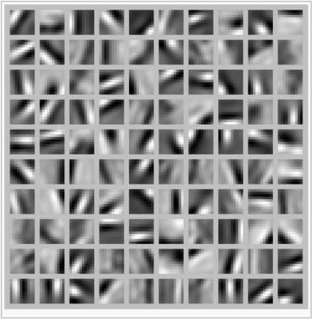
display a random sample of 204 patches from the dataset

以下是一些设置参数，就是学习单个自动编码器，学到一个隐含层的基（参数W，b）。

visibleSize = 8*8; % number of input units

hiddenSize = 25; % number of hidden units

sparsityParam = 0.01; % desired average activation of the hidden units.

% (This was denoted by the Greek alphabet rho, which looks like a lower-case "p",

% in the lecture notes).

lambda = 0.0001; % weight decay parameter

beta = 3; % weight of sparsity penalty term

以下是序列输出结果

>> train

Iteration FunEvals Step Length Function Val Opt Cond

1 3 8.63782e-03 3.98056e+01 1.03759e+03

2 4 1.00000e+00 6.68382e+00 2.49253e+02

…….

399 414 1.00000e+00 4.49948e-01 1.45238e-02

400 415 1.00000e+00 4.49947e-01 1.40765e-02

Exceeded Maximum Number of Iterations

时间已过 20.942873 秒。

教程中说Our implementation took around 5 minutes to run on a fast computer.

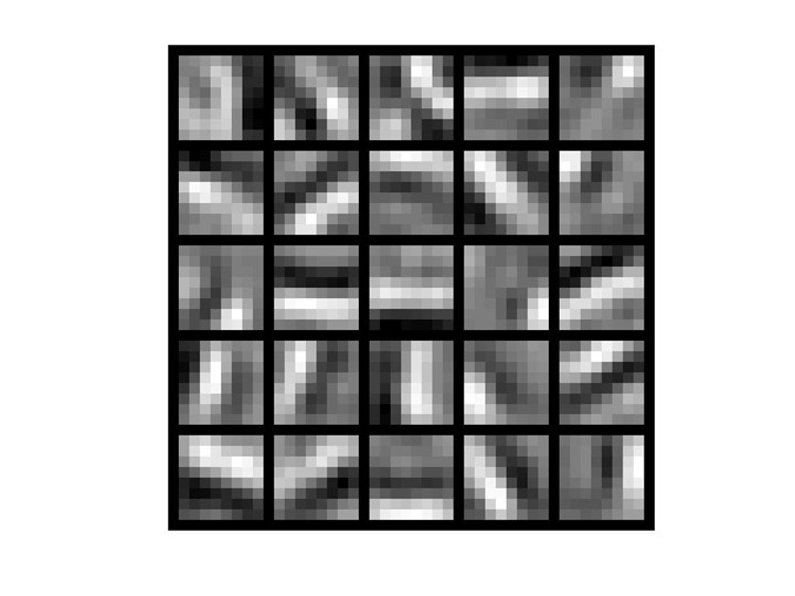
sparse autoencoder algorithm learning a set of edge detectors.

隐藏层权重可视化后，我们可以看出学到了一组边缘检测器，一组基或称字典。

练习代码：

train

%% CS294A/CS294W Programming Assignment Starter Code

%  Instructions
%  ------------
% 
%  This file contains code that helps you get started on the
%  programming assignment. You will need to complete the code in sampleIMAGES.m,
%  sparseAutoencoderCost.m and computeNumericalGradient.m. 
%  For the purpose of completing the assignment, you do not need to
%  change the code in this file. 
%
%%======================================================================
%% STEP 0: Here we provide the relevant parameters values that will
%  allow your sparse autoencoder to get good filters; you do not need to 
%  change the parameters below.

visibleSize = 8*8;   % number of input units 
hiddenSize = 25;     % number of hidden units 
sparsityParam = 0.01;   % desired average activation of the hidden units.
                     % (This was denoted by the Greek alphabet rho, which looks like a lower-case "p",
             %  in the lecture notes). 
lambda = 0.0001;     % weight decay parameter       
beta = 3;            % weight of sparsity penalty term       

%%======================================================================
%% STEP 1: Implement sampleIMAGES
%
%  After implementing sampleIMAGES, the display_network command should
%  display a random sample of 200 patches from the dataset

patches = sampleIMAGES;
display_network(patches(:,randi(size(patches,2),204,1)),8);


%  Obtain random parameters theta
theta = initializeParameters(hiddenSize, visibleSize);

%%======================================================================
%% STEP 2: Implement sparseAutoencoderCost
%
%  You can implement all of the components (squared error cost, weight decay term,
%  sparsity penalty) in the cost function at once, but it may be easier to do 
%  it step-by-step and run gradient checking (see STEP 3) after each step.  We 
%  suggest implementing the sparseAutoencoderCost function using the following steps:
%
%  (a) Implement forward propagation in your neural network, and implement the 
%      squared error term of the cost function.  Implement backpropagation to 
%      compute the derivatives.   Then (using lambda=beta=0), run Gradient Checking 
%      to verify that the calculations corresponding to the squared error cost 
%      term are correct.
%
%  (b) Add in the weight decay term (in both the cost function and the derivative
%      calculations), then re-run Gradient Checking to verify correctness. 
%
%  (c) Add in the sparsity penalty term, then re-run Gradient Checking to 
%      verify correctness.
%
%  Feel free to change the training settings when debugging your
%  code.  (For example, reducing the training set size or 
%  number of hidden units may make your code run faster; and setting beta 
%  and/or lambda to zero may be helpful for debugging.)  However, in your 
%  final submission of the visualized weights, please use parameters we 
%  gave in Step 0 above.
[cost, grad] = sparseAutoencoderCost(theta, visibleSize, hiddenSize, lambda, ...
                                     sparsityParam, beta, patches);

%%======================================================================
%% STEP 3: Gradient Checking
%
% Hint: If you are debugging your code, performing gradient checking on smaller models 
% and smaller training sets (e.g., using only 10 training examples and 1-2 hidden 
% units) may speed things up.

% First, lets make sure your numerical gradient computation is correct for a
% simple function.  After you have implemented computeNumericalGradient.m,
% run the following: 
% checkNumericalGradient();
% 
% % Now we can use it to check your cost function and derivative calculations
% % for the sparse autoencoder.  
% numgrad = computeNumericalGradient( @(x) sparseAutoencoderCost(x, visibleSize, ...
%                                                   hiddenSize, lambda, ...
%                                                   sparsityParam, beta, ...
%                                                   patches), theta);
% 
% % Use this to visually compare the gradients side by side
% disp([numgrad grad]); 
% 
% % Compare numerically computed gradients with the ones obtained from backpropagation
% diff = norm(numgrad-grad)/norm(numgrad+grad);
% disp(diff); % Should be small. In our implementation, these values are
%             % usually less than 1e-9.
% 
%             % When you got this working, Congratulations!!! 

%%======================================================================
%% STEP 4: After verifying that your implementation of
%  sparseAutoencoderCost is correct, You can start training your sparse
%  autoencoder with minFunc (L-BFGS).

%  Randomly initialize the parameters
theta = initializeParameters(hiddenSize, visibleSize);

%  Use minFunc to minimize the function
addpath minFunc/
options.Method = 'lbfgs'; % Here, we use L-BFGS to optimize our cost
                          % function. Generally, for minFunc to work, you
                          % need a function pointer with two outputs: the
                          % function value and the gradient. In our problem,
                          % sparseAutoencoderCost.m satisfies this.
options.maxIter = 400;      % Maximum number of iterations of L-BFGS to run 
options.display = 'on';


[opttheta, cost] = minFunc( @(p) sparseAutoencoderCost(p, ...
                                   visibleSize, hiddenSize, ...
                                   lambda, sparsityParam, ...
                                   beta, patches), ...
                              theta, options);

%%======================================================================
%% STEP 5: Visualization 

W1 = reshape(opttheta(1:hiddenSize*visibleSize), hiddenSize, visibleSize);
display_network(W1', 12); 

print -djpeg weights.jpg   % save the visualization to a file 

sampleIMAGES

function patches = sampleIMAGES()
% sampleIMAGES
% Returns 10000 patches for training

load IMAGES;    % load images from disk 

patchsize = 8;  % we'll use 8x8 patches 
numpatches = 10000;

% Initialize patches with zeros.  Your code will fill in this matrix--one
% column per patch, 10000 columns. 
patches = zeros(patchsize*patchsize, numpatches);

%% ---------- YOUR CODE HERE --------------------------------------
%  Instructions: Fill in the variable called "patches" using data 
%  from IMAGES.  
%  
%  IMAGES is a 3D array containing 10 images
%  For instance, IMAGES(:,:,6) is a 512x512 array containing the 6th image,
%  and you can type "imagesc(IMAGES(:,:,6)), colormap gray;" to visualize
%  it. (The contrast on these images look a bit off because they have
%  been preprocessed using using "whitening."  See the lecture notes for
%  more details.) As a second example, IMAGES(21:30,21:30,1) is an image
%  patch corresponding to the pixels in the block (21,21) to (30,30) of
%  Image 1

for imageNum = 1 : 10
    image = IMAGES(:, :, imageNum);
    [rowNum, colNum] = size(image);
    
    for patchNum = 1 : 1000
        xPos = randi(rowNum - patchsize + 1);
        yPos = randi(colNum - patchsize + 1);
        patches(:, 1000 * (imageNum - 1) + patchNum) = ...
            reshape(image(xPos : xPos + 7, yPos : yPos + 7), 64, 1);
    end
    
end








%% ---------------------------------------------------------------
% For the autoencoder to work well we need to normalize the data
% Specifically, since the output of the network is bounded between [0,1]
% (due to the sigmoid activation function), we have to make sure 
% the range of pixel values is also bounded between [0,1]
patches = normalizeData(patches);

end


%% ---------------------------------------------------------------
function patches = normalizeData(patches)

% Squash data to [0.1, 0.9] since we use sigmoid as the activation
% function in the output layer

% Remove DC (mean of images). 
patches = bsxfun(@minus, patches, mean(patches));

% Truncate to +/-3 standard deviations and scale to -1 to 1
pstd = 3 * std(patches(:));
patches = max(min(patches, pstd), -pstd) / pstd;

% Rescale from [-1,1] to [0.1,0.9]
patches = (patches + 1) * 0.4 + 0.1;

end

sparseAutoencoderCost

function [cost,grad] = sparseAutoencoderCost(theta, visibleSize, hiddenSize, ...
                                             lambda, sparsityParam, beta, data)

% visibleSize: the number of input units (probably 64) 
% hiddenSize: the number of hidden units (probably 25) 
% lambda: weight decay parameter
% sparsityParam: The desired average activation for the hidden units (denoted in the lecture
%                           notes by the greek alphabet rho, which looks like a lower-case "p").
% beta: weight of sparsity penalty term
% data: Our 64x10000 matrix containing the training data.  So, data(:,i) is the i-th training example. 
  
% The input theta is a vector (because minFunc expects the parameters to be a vector). 
% We first convert theta to the (W1, W2, b1, b2) matrix/vector format, so that this 
% follows the notation convention of the lecture notes. 

W1 = reshape(theta(1:hiddenSize*visibleSize), hiddenSize, visibleSize);
W2 = reshape(theta(hiddenSize*visibleSize+1:2*hiddenSize*visibleSize), visibleSize, hiddenSize);
b1 = theta(2*hiddenSize*visibleSize+1:2*hiddenSize*visibleSize+hiddenSize);
b2 = theta(2*hiddenSize*visibleSize+hiddenSize+1:end);

% Cost and gradient variables (your code needs to compute these values). 
% Here, we initialize them to zeros. 
cost = 0;
W1grad = zeros(size(W1)); 
W2grad = zeros(size(W2));
b1grad = zeros(size(b1)); 
b2grad = zeros(size(b2));

%% ---------- YOUR CODE HERE --------------------------------------
%  Instructions: Compute the cost/optimization objective J_sparse(W,b) for the Sparse Autoencoder,
%                and the corresponding gradients W1grad, W2grad, b1grad, b2grad.
%
% W1grad, W2grad, b1grad and b2grad should be computed using backpropagation.
% Note that W1grad has the same dimensions as W1, b1grad has the same dimensions
% as b1, etc.  Your code should set W1grad to be the partial derivative of J_sparse(W,b) with
% respect to W1.  I.e., W1grad(i,j) should be the partial derivative of J_sparse(W,b) 
% with respect to the input parameter W1(i,j).  Thus, W1grad should be equal to the term 
% [(1/m) Delta W^{(1)} + lambda W^{(1)}] in the last block of pseudo-code in Section 2.2 
% of the lecture notes (and similarly for W2grad, b1grad, b2grad).
% 
% Stated differently, if we were using batch gradient descent to optimize the parameters,
% the gradient descent update to W1 would be W1 := W1 - alpha * W1grad, and similarly for W2, b1, b2. 
% 

Jcost = 0;
Jweight = 0;
Jsparse = 0;
[n m] = size(data);


z2 = W1*data+repmat(b1,1,m);
a2 = sigmoid(z2);
z3 = W2*a2+repmat(b2,1,m);
a3 = sigmoid(z3);

Jcost = (0.5/m)*sum(sum((a3-data).^2));

Jweight = (1/2)*(sum(sum(W1.^2))+sum(sum(W2.^2)));

rho = (1/m).*sum(a2,2);
Jsparse = sum(sparsityParam.*log(sparsityParam./rho)+ ...
        (1-sparsityParam).*log((1-sparsityParam)./(1-rho)));

cost = Jcost+lambda*Jweight+beta*Jsparse;

d3 = -(data-a3).*dsigmoid(a3);
sterm = beta*(-sparsityParam./rho+(1-sparsityParam)./(1-rho));

d2 = (W2'*d3+repmat(sterm,1,m)).*dsigmoid(a2); 

W1grad = W1grad+d2*data';
W1grad = (1/m)*W1grad+lambda*W1;

W2grad = W2grad+d3*a2';
W2grad = (1/m).*W2grad+lambda*W2;

b1grad = b1grad+sum(d2,2);
b1grad = (1/m)*b1grad;

b2grad = b2grad+sum(d3,2);
b2grad = (1/m)*b2grad;

%-------------------------------------------------------------------
% After computing the cost and gradient, we will convert the gradients back
% to a vector format (suitable for minFunc).  Specifically, we will unroll
% your gradient matrices into a vector.

grad = [W1grad(:) ; W2grad(:) ; b1grad(:) ; b2grad(:)];

end

%-------------------------------------------------------------------
% Here's an implementation of the sigmoid function, which you may find useful
% in your computation of the costs and the gradients.  This inputs a (row or
% column) vector (say (z1, z2, z3)) and returns (f(z1), f(z2), f(z3)). 

function sigm = sigmoid(x)
  
    sigm = 1 ./ (1 + exp(-x));
end

function dsigm = dsigmoid(a)
dsigm = a .* (1.0 - a);
end

computeNumericalGradient

function numgrad = computeNumericalGradient(J, theta)
% numgrad = computeNumericalGradient(J, theta)
% theta: a vector of parameters
% J: a function that outputs a real-number. Calling y = J(theta) will return the
% function value at theta. 
  
% Initialize numgrad with zeros
numgrad = zeros(size(theta));

%% ---------- YOUR CODE HERE --------------------------------------
% Instructions: 
% Implement numerical gradient checking, and return the result in numgrad.  
% (See Section 2.3 of the lecture notes.)
% You should write code so that numgrad(i) is (the numerical approximation to) the 
% partial derivative of J with respect to the i-th input argument, evaluated at theta.  
% I.e., numgrad(i) should be the (approximately) the partial derivative of J with 
% respect to theta(i).
%                
% Hint: You will probably want to compute the elements of numgrad one at a time. 

epsilon = 1e-4;
n = size(theta,1);
E = eye(n);
for i = 1:n
    delta = E(:,i)*epsilon;
    numgrad(i) = (J(theta+delta)-J(theta-delta))/(epsilon*2.0);
end

%% ---------------------------------------------------------------
end

---

声明：
不要将本博客用作为商业目的，并且本人博客使用的内容仅仅作为个人学习，其中包括引用的或没找到出处而未引用的内容。
转载请注明，本文地址：http://www.cnblogs.com/JayZen/p/4129386.html 

参考：

UFLDL教程

Hugo Larochelle nn course