3.8 多层感知机
以多层感知机(MLP)为例,介绍多层神经网络的概念。
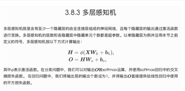
3.8.1 隐藏层
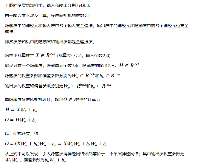
多层感知机在单层神经网络的基础上引入了一到多个隐藏层。隐藏层位于输入层和输出层之间。
下图展示一个多层感知机的神经网络图,它含有一个隐藏层,该层具有5个隐藏单元。

3.8.2 激活函数
上述问题的根源在于全连接层只是对数据进行了仿射变换,而多个仿射变换的叠加仍然是一个仿射变换。
解决问题的方法在于引入非线性变换(如对隐藏变量按元素运算的非线性函数进行变换,再作为下一个全连接层的输入)。
以上用于操作的非线性函数叫做激活函数。
3.8.2.1 ReLU函数
%matplotlib inline
import torch
import numpy as np
import matplotlib.pylab as plt
import sys
sys.path.append('D:Anaconda3envspytorchLib')
import d2lzh_pytorch as d2l

def xyplot(x_vals,y_vals,name):
    d2l.set_figsize(figsize = (5,2.5))
    d2l.plt.plot(x_vals.detach().numpy(),y_vals.detach().numpy())
    d2l.plt.xlabel('x')
    d2l.plt.ylabel(name+'(x)')
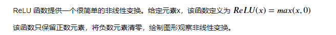
绘制ReLU函数,该激活函数是一个两段线性函数
x = torch.arange(-8.0,8.0,0.1,requires_grad=True)
y = x.relu()
xyplot(x,y,'relu')
如上图所示,输入为负数时,ReLU函数的导数为0;输入为正数时,ReLU函数的导数为1。
尽管输入为0时ReLU函数不可导,但是我们可以取此处的到导数为0。
绘制ReLU函数的导数。
y.sum().backward()
xyplot(x,x.grad,'grad of relu')

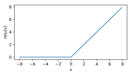
3.8.2.2 sigmoid函数

y = x.sigmoid()
xyplot(x,y,'sigmoid')
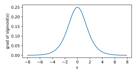
绘制sigmoid函数的导数
x.grad.zero_()
y.sum().backward()
xyplot(x,x.grad,'grad of sigmoid')
3.8.2.3 tanh函数
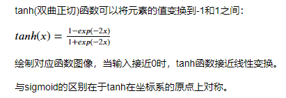
y = x.tanh()
xyplot(x,y,'tanh')

绘制其对应导数图像
x.grad.zero_()
y.sum().backward()
xyplot(x,x.grad,'grad of tanh')

回顾
3.9 多层感知机的从零开始实现
导包
import torch
import numpy as np
import sys
sys.path.append("D:Anaconda3envspytorchLib")
import d2lzh_pytorch as d2l

print(torch.__version__)
1.8.1
3.9.1 获取和读取数据
这里继续使用 Fashion-MNIST 数据集。使用多层感知机对图像进行分类
batch_size = 256
train_iter, test_iter = d2l.load_data_fashion_mnist(batch_size)
3.9.2 定义模型参数
Fashion-MNIST 数据集中图像形状为 28×28,类别数为10。
此处使用长度 28×28 = 784 的向量表示每一张图像。即输入个数为784,输出个数为10。
实验中设超参数隐藏单元个数为256.
num_inputs, num_outputs, num_hiddens = 784, 10, 256

W1 = torch.tensor(np.random.normal(0, 0.01, (num_inputs, num_hiddens)), dtype=torch.float)
b1 = torch.zeros(num_hiddens, dtype=torch.float)
W2 = torch.tensor(np.random.normal(0, 0.01, (num_hiddens, num_outputs)), dtype=torch.float)
b2 = torch.zeros(num_outputs, dtype=torch.float)

params = [W1, b1, W2, b2]
for param in params:
    param.requires_grad_(requires_grad=True)
3.9.3 定义激活函数
使用基础max函数实现ReLU,不直接调用relu函数
def relu(X):
    return torch.max(input=X, other=torch.tensor(0.0))
3.9.4 定义模型
同softmax回归一样,我们通过view函数将每张原始图像改变成长度为num_inputs的向量,实现多层感知机的计算表达式。
def net(X):
    X = X.view((-1, num_inputs))
    H = relu(torch.matmul(X, W1) + b1)
    return torch.matmul(H, W2) + b2
3.9.5 定义损失函数
直接使用PyTorch提供的包括softmax运算和交叉熵损失计算的函数
loss = torch.nn.CrossEntropyLoss()
3.9.6 训练模型
直接调用d2lzh_pytorch包中的train_ch3函数。
设超参数迭代周期数为5,学习率为100.0
num_epochs, lr = 5, 100.0
d2l.train_ch3(net, train_iter, test_iter, loss, num_epochs, batch_size, params, lr)
epoch 1, loss 0.0030, train acc 0.711, test acc 0.796
epoch 2, loss 0.0019, train acc 0.823, test acc 0.735
epoch 3, loss 0.0017, train acc 0.843, test acc 0.841
epoch 4, loss 0.0015, train acc 0.856, test acc 0.837
epoch 5, loss 0.0014, train acc 0.864, test acc 0.858
3.10 多层感知机的简洁实现
使用Gluon实现上一节中的多层感知机
导包
import torch
from torch import nn
from torch.nn import init
import numpy as np
import sys
sys.path.append("D:Anaconda3envspytorchLib")
import d2lzh_pytorch as d2l
3.10.1 定义模型
与softmax回归不同点在于多加了一个全连接层作为隐藏层。它的隐藏单元个数为256,使用ReLU函数作为激活函数
num_inputs,num_outputs,num_hiddens = 784,10,256

net = nn.Sequential(
    d2l.FlattenLayer(),
    nn.Linear(num_inputs,num_hiddens),
    nn.ReLU(),
    nn.Linear(num_hiddens,num_outputs)
    )

for params in net.parameters():
    init.normal_(params,mean = 0,std = 0.01)
3.10.2 读取数据并训练模型
使用softmax回归相同步骤读取数据并训练模型
注:这里使用的Pytorch中的SGD并非d2lzh_pytorch中的sgd,不存在学习率大的问题
batch_size = 256
train_iter,test_iter = d2l.load_data_fashion_mnist(batch_size)
loss = torch.nn.CrossEntropyLoss()

optimizer = torch.optim.SGD(net.parameters(),lr = 0.5)

num_epochs = 5
d2l.train_ch3(net,train_iter,test_iter,loss,num_epochs,batch_size,None,None,optimizer)
epoch 1, loss 0.0032, train acc 0.693, test acc 0.813
epoch 2, loss 0.0019, train acc 0.818, test acc 0.771
epoch 3, loss 0.0017, train acc 0.843, test acc 0.802
epoch 4, loss 0.0015, train acc 0.854, test acc 0.854
epoch 5, loss 0.0014, train acc 0.865, test acc 0.803