Coggle 30 Days of ML：结构化赛题：天池二手车交易价格预测（一）

任务1：报名比赛，下载比赛数据集并完成读取

载入各种数据科学以及可视化库

import warnings
warnings.filterwarnings('ignore')#忽略版本问题警告

import numpy as np
import pandas as pd
import matplotlib.pyplot as plt
import seaborn as sns
import missingno as msno#缺失值可视化Python工具库
from scipy import stats

使用Pandas完成数据集读取

Train_data = pd.read_csv('used_car_train_20200313.csv',sep = ' ')
Test_data = pd.read_csv('used_car_testB_20200421.csv',sep = ' ')

##简要观察头尾训练数据
Train_data.head().append(Train_data.tail())

	SaleID	name	regDate	model	brand	bodyType	fuelType	gearbox	power	kilometer	...	v_5	v_6	v_7	v_8	v_9	v_10	v_11	v_12	v_13	v_14
0	0	736	20040402	30.0	6	1.0	0.0	0.0	60	12.5	...	0.235676	0.101988	0.129549	0.022816	0.097462	-2.881803	2.804097	-2.420821	0.795292	0.914762
1	1	2262	20030301	40.0	1	2.0	0.0	0.0	0	15.0	...	0.264777	0.121004	0.135731	0.026597	0.020582	-4.900482	2.096338	-1.030483	-1.722674	0.245522
2	2	14874	20040403	115.0	15	1.0	0.0	0.0	163	12.5	...	0.251410	0.114912	0.165147	0.062173	0.027075	-4.846749	1.803559	1.565330	-0.832687	-0.229963
3	3	71865	19960908	109.0	10	0.0	0.0	1.0	193	15.0	...	0.274293	0.110300	0.121964	0.033395	0.000000	-4.509599	1.285940	-0.501868	-2.438353	-0.478699
4	4	111080	20120103	110.0	5	1.0	0.0	0.0	68	5.0	...	0.228036	0.073205	0.091880	0.078819	0.121534	-1.896240	0.910783	0.931110	2.834518	1.923482
149995	149995	163978	20000607	121.0	10	4.0	0.0	1.0	163	15.0	...	0.280264	0.000310	0.048441	0.071158	0.019174	1.988114	-2.983973	0.589167	-1.304370	-0.302592
149996	149996	184535	20091102	116.0	11	0.0	0.0	0.0	125	10.0	...	0.253217	0.000777	0.084079	0.099681	0.079371	1.839166	-2.774615	2.553994	0.924196	-0.272160
149997	149997	147587	20101003	60.0	11	1.0	1.0	0.0	90	6.0	...	0.233353	0.000705	0.118872	0.100118	0.097914	2.439812	-1.630677	2.290197	1.891922	0.414931
149998	149998	45907	20060312	34.0	10	3.0	1.0	0.0	156	15.0	...	0.256369	0.000252	0.081479	0.083558	0.081498	2.075380	-2.633719	1.414937	0.431981	-1.659014
149999	149999	177672	19990204	19.0	28	6.0	0.0	1.0	193	12.5	...	0.284475	0.000000	0.040072	0.062543	0.025819	1.978453	-3.179913	0.031724	-1.483350	-0.342674

10 rows × 31 columns

任务2：对数据字段进行理解，并对特征字段依次进行数据分析

使用Pandas对比赛数据集进行分析

分析每个字段的取值、范围和类型

使用describe观察每列取值范围和统计量

Train_data.describe()

	SaleID	name	regDate	model	brand	bodyType	fuelType	gearbox	power	kilometer	...	v_5	v_6	v_7	v_8	v_9	v_10	v_11	v_12	v_13	v_14
count	150000.000000	150000.000000	1.500000e+05	149999.000000	150000.000000	145494.000000	141320.000000	144019.000000	150000.000000	150000.000000	...	150000.000000	150000.000000	150000.000000	150000.000000	150000.000000	150000.000000	150000.000000	150000.000000	150000.000000	150000.000000
mean	74999.500000	68349.172873	2.003417e+07	47.129021	8.052733	1.792369	0.375842	0.224943	119.316547	12.597160	...	0.248204	0.044923	0.124692	0.058144	0.061996	-0.001000	0.009035	0.004813	0.000313	-0.000688
std	43301.414527	61103.875095	5.364988e+04	49.536040	7.864956	1.760640	0.548677	0.417546	177.168419	3.919576	...	0.045804	0.051743	0.201410	0.029186	0.035692	3.772386	3.286071	2.517478	1.288988	1.038685
min	0.000000	0.000000	1.991000e+07	0.000000	0.000000	0.000000	0.000000	0.000000	0.000000	0.500000	...	0.000000	0.000000	0.000000	0.000000	0.000000	-9.168192	-5.558207	-9.639552	-4.153899	-6.546556
25%	37499.750000	11156.000000	1.999091e+07	10.000000	1.000000	0.000000	0.000000	0.000000	75.000000	12.500000	...	0.243615	0.000038	0.062474	0.035334	0.033930	-3.722303	-1.951543	-1.871846	-1.057789	-0.437034
50%	74999.500000	51638.000000	2.003091e+07	30.000000	6.000000	1.000000	0.000000	0.000000	110.000000	15.000000	...	0.257798	0.000812	0.095866	0.057014	0.058484	1.624076	-0.358053	-0.130753	-0.036245	0.141246
75%	112499.250000	118841.250000	2.007111e+07	66.000000	13.000000	3.000000	1.000000	0.000000	150.000000	15.000000	...	0.265297	0.102009	0.125243	0.079382	0.087491	2.844357	1.255022	1.776933	0.942813	0.680378
max	149999.000000	196812.000000	2.015121e+07	247.000000	39.000000	7.000000	6.000000	1.000000	19312.000000	15.000000	...	0.291838	0.151420	1.404936	0.160791	0.222787	12.357011	18.819042	13.847792	11.147669	8.658418

8 rows × 30 columns

Test_data.describe()

	SaleID	name	regDate	model	brand	bodyType	fuelType	gearbox	power	kilometer	...	v_5	v_6	v_7	v_8	v_9	v_10	v_11	v_12	v_13	v_14
count	50000.000000	50000.000000	5.000000e+04	50000.00000	50000.000000	48496.000000	47076.000000	48032.000000	50000.000000	50000.000000	...	50000.000000	50000.000000	50000.000000	50000.000000	50000.000000	50000.000000	50000.000000	50000.000000	50000.000000	50000.000000
mean	224999.500000	68505.606100	2.003401e+07	47.64948	8.087140	1.793736	0.376498	0.226953	119.766960	12.598260	...	0.248147	0.044624	0.124693	0.058198	0.062113	0.019633	0.002759	0.004342	0.004570	-0.007209
std	14433.901067	61032.124271	5.351615e+04	49.90741	7.899648	1.764970	0.549281	0.418866	206.313348	3.912519	...	0.045836	0.051664	0.201440	0.029171	0.035723	3.764095	3.289523	2.515912	1.287194	1.044718
min	200000.000000	1.000000	1.991000e+07	0.00000	0.000000	0.000000	0.000000	0.000000	0.000000	0.500000	...	0.000000	0.000000	0.000000	0.000000	0.000000	-9.119719	-5.662163	-8.291868	-4.157649	-6.098192
25%	212499.750000	11315.000000	1.999100e+07	11.00000	1.000000	0.000000	0.000000	0.000000	75.000000	12.500000	...	0.243436	0.000035	0.062519	0.035413	0.033880	-3.675196	-1.963928	-1.865406	-1.048722	-0.440706
50%	224999.500000	52215.000000	2.003091e+07	30.00000	6.000000	1.000000	0.000000	0.000000	110.000000	15.000000	...	0.257818	0.000801	0.095880	0.056804	0.058749	1.632134	-0.375537	-0.138943	-0.036352	0.136849
75%	237499.250000	118710.750000	2.007110e+07	66.00000	13.000000	3.000000	1.000000	0.000000	150.000000	15.000000	...	0.265263	0.101654	0.125470	0.079387	0.087624	2.846205	1.263451	1.775632	0.945239	0.685555
max	249999.000000	196808.000000	2.015121e+07	246.00000	39.000000	7.000000	6.000000	1.000000	19211.000000	15.000000	...	0.291176	0.153403	1.411559	0.157458	0.211304	12.177864	18.789496	13.384828	5.635374	2.649768

8 rows × 29 columns

使用info查看字段类型

Train_data.info()

<class 'pandas.core.frame.DataFrame'>
RangeIndex: 150000 entries, 0 to 149999
Data columns (total 31 columns):
 #   Column             Non-Null Count   Dtype  
---  ------             --------------   -----  
 0   SaleID             150000 non-null  int64  
 1   name               150000 non-null  int64  
 2   regDate            150000 non-null  int64  
 3   model              149999 non-null  float64
 4   brand              150000 non-null  int64  
 5   bodyType           145494 non-null  float64
 6   fuelType           141320 non-null  float64
 7   gearbox            144019 non-null  float64
 8   power              150000 non-null  int64  
 9   kilometer          150000 non-null  float64
 10  notRepairedDamage  150000 non-null  object 
 11  regionCode         150000 non-null  int64  
 12  seller             150000 non-null  int64  
 13  offerType          150000 non-null  int64  
 14  creatDate          150000 non-null  int64  
 15  price              150000 non-null  int64  
 16  v_0                150000 non-null  float64
 17  v_1                150000 non-null  float64
 18  v_2                150000 non-null  float64
 19  v_3                150000 non-null  float64
 20  v_4                150000 non-null  float64
 21  v_5                150000 non-null  float64
 22  v_6                150000 non-null  float64
 23  v_7                150000 non-null  float64
 24  v_8                150000 non-null  float64
 25  v_9                150000 non-null  float64
 26  v_10               150000 non-null  float64
 27  v_11               150000 non-null  float64
 28  v_12               150000 non-null  float64
 29  v_13               150000 non-null  float64
 30  v_14               150000 non-null  float64
dtypes: float64(20), int64(10), object(1)
memory usage: 35.5+ MB

Test_data.info()

<class 'pandas.core.frame.DataFrame'>
RangeIndex: 50000 entries, 0 to 49999
Data columns (total 30 columns):
 #   Column             Non-Null Count  Dtype  
---  ------             --------------  -----  
 0   SaleID             50000 non-null  int64  
 1   name               50000 non-null  int64  
 2   regDate            50000 non-null  int64  
 3   model              50000 non-null  float64
 4   brand              50000 non-null  int64  
 5   bodyType           48496 non-null  float64
 6   fuelType           47076 non-null  float64
 7   gearbox            48032 non-null  float64
 8   power              50000 non-null  int64  
 9   kilometer          50000 non-null  float64
 10  notRepairedDamage  50000 non-null  object 
 11  regionCode         50000 non-null  int64  
 12  seller             50000 non-null  int64  
 13  offerType          50000 non-null  int64  
 14  creatDate          50000 non-null  int64  
 15  v_0                50000 non-null  float64
 16  v_1                50000 non-null  float64
 17  v_2                50000 non-null  float64
 18  v_3                50000 non-null  float64
 19  v_4                50000 non-null  float64
 20  v_5                50000 non-null  float64
 21  v_6                50000 non-null  float64
 22  v_7                50000 non-null  float64
 23  v_8                50000 non-null  float64
 24  v_9                50000 non-null  float64
 25  v_10               50000 non-null  float64
 26  v_11               50000 non-null  float64
 27  v_12               50000 non-null  float64
 28  v_13               50000 non-null  float64
 29  v_14               50000 non-null  float64
dtypes: float64(20), int64(9), object(1)
memory usage: 11.4+ MB

结合比赛页面中具体字段的含义，对字段的取值分布进行分析

提取数值类型特征列名

#提取数值类型列
numerical_cols = Train_data.select_dtypes(exclude='object').columns

#提取特征列
feature_cols = [col for col in numerical_cols if col not in ['SaleID','name','regDate','creatDate','price','model','brand','regionCode','seller']]

feature_cols = [col for col in feature_cols if 'Type' not in col]

feature_cols

['gearbox',
 'power',
 'kilometer',
 'v_0',
 'v_1',
 'v_2',
 'v_3',
 'v_4',
 'v_5',
 'v_6',
 'v_7',
 'v_8',
 'v_9',
 'v_10',
 'v_11',
 'v_12',
 'v_13',
 'v_14']

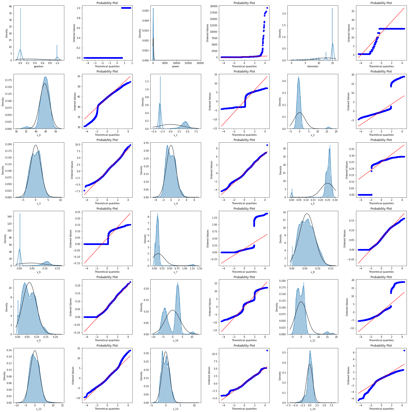
采用直方图加Q-Q图的形式对特征列数据字段取值分布进行分析

train_cols = 6
train_rows = len(feature_cols)
plt.figure(figsize = (4*train_cols,4*train_rows))

i = 0
for col in feature_cols:
    i+=1
    ax = plt.subplot(train_rows,train_cols,i)
    #拟合正态分布
    sns.distplot(Train_data[col],fit = stats.norm)
    
    i+=1
    ax = plt.subplot(train_rows,train_cols,i)
    res = stats.probplot(Train_data[col],plot = plt)
plt.tight_layout()
plt.show()

​

​

test_cols = 6
test_rows = len(feature_cols)
plt.figure(figsize = (4*test_cols,4*test_rows))

i = 0
for col in feature_cols:
    i+=1
    ax = plt.subplot(test_rows,test_cols,i)
    #拟合正态分布
    sns.distplot(Test_data[col],fit = stats.norm)
    
    i+=1
    ax = plt.subplot(train_rows,train_cols,i)
    res = stats.probplot(Test_data[col],plot = plt)
plt.tight_layout()
plt.show()

​

​

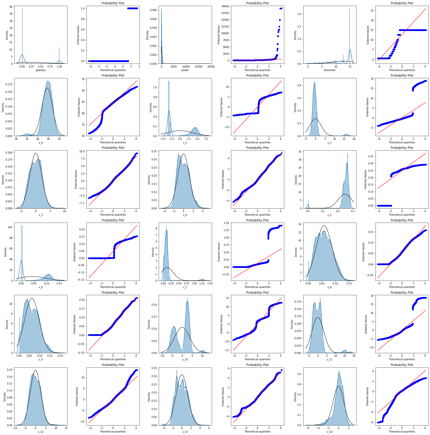
发现特征变量v_0,v_3,v_4,v_8,v_9,v_12,v_13,v_14的取值能较好地服从正态分布

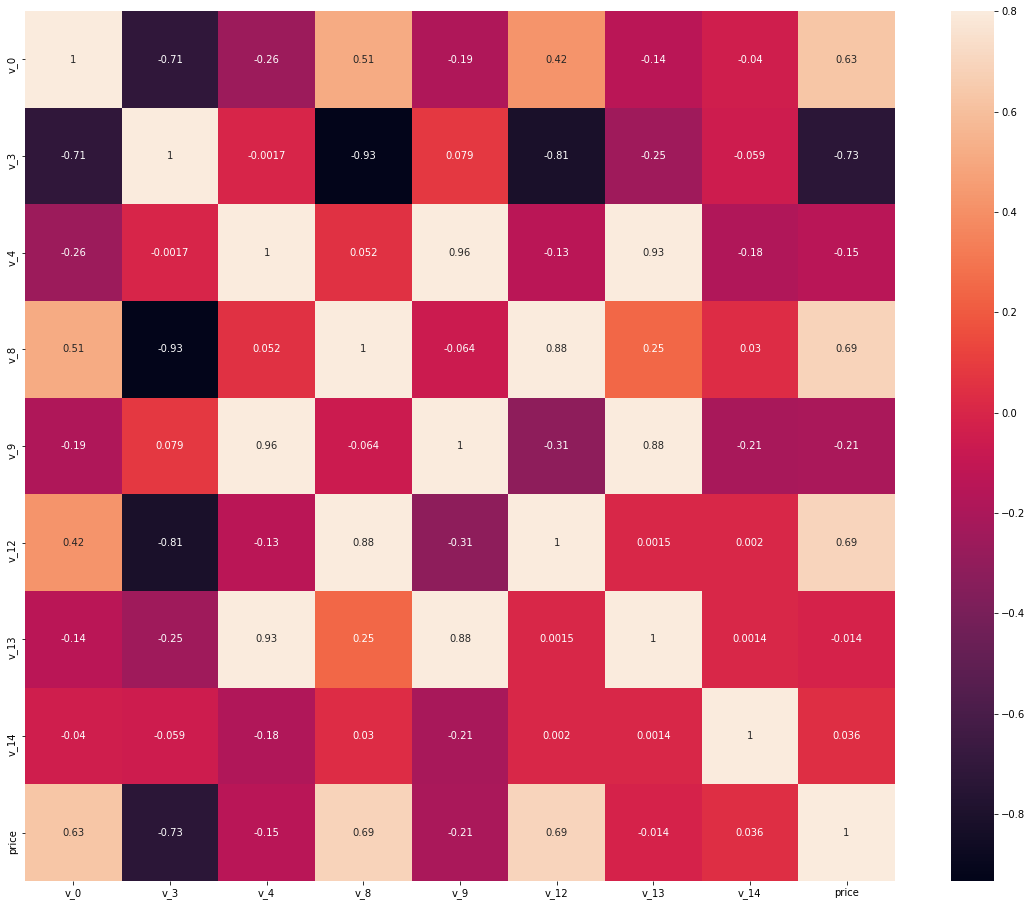
计算特征字段与标签的相关性

保留较好符合正态分布的特征变量

data_train = Train_data[['v_0','v_3','v_4','v_8','v_9','v_12','v_13','v_14','price']]
data_test = Test_data[['v_0','v_3','v_4','v_8','v_9','v_12','v_13','v_14']]

计算相关性并绘制热力图

train_corr = data_train.corr()
train_corr

	v_0	v_3	v_4	v_8	v_9	v_12	v_13	v_14	price
v_0	1.000000	-0.710480	-0.259714	0.514149	-0.186243	0.415711	-0.136938	-0.039809	0.628397
v_3	-0.710480	1.000000	-0.001694	-0.933161	0.079292	-0.811301	-0.246052	-0.058561	-0.730946
v_4	-0.259714	-0.001694	1.000000	0.051741	0.962928	-0.134611	0.934580	-0.178518	-0.147085
v_8	0.514149	-0.933161	0.051741	1.000000	-0.063577	0.882121	0.250423	0.030416	0.685798
v_9	-0.186243	0.079292	0.962928	-0.063577	1.000000	-0.313634	0.880545	-0.214151	-0.206205
v_12	0.415711	-0.811301	-0.134611	0.882121	-0.313634	1.000000	0.001512	0.002045	0.692823
v_13	-0.136938	-0.246052	0.934580	0.250423	0.880545	0.001512	1.000000	0.001419	-0.013993
v_14	-0.039809	-0.058561	-0.178518	0.030416	-0.214151	0.002045	0.001419	1.000000	0.035911
price	0.628397	-0.730946	-0.147085	0.685798	-0.206205	0.692823	-0.013993	0.035911	1.000000

ax = plt.subplots(figsize = (20,16))
ax = sns.heatmap(train_corr,vmax = .8,square = True,annot = True)

​

​

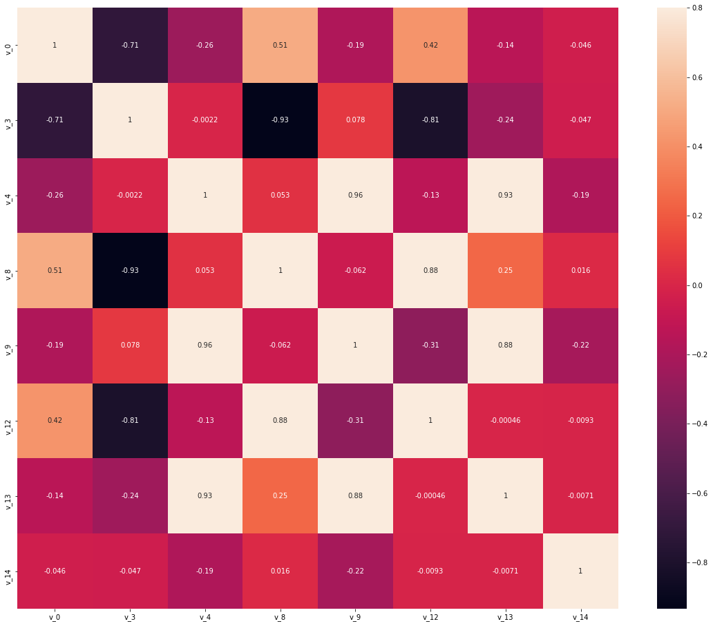
test_corr = data_test.corr()
test_corr

	v_0	v_3	v_4	v_8	v_9	v_12	v_13	v_14
v_0	1.000000	-0.710375	-0.260180	0.514193	-0.185413	0.415299	-0.140730	-0.045889
v_3	-0.710375	1.000000	-0.002159	-0.933028	0.078054	-0.810487	-0.242746	-0.047387
v_4	-0.260180	-0.002159	1.000000	0.053027	0.963043	-0.131721	0.934898	-0.187063
v_8	0.514193	-0.933028	0.053027	1.000000	-0.061830	0.882173	0.247377	0.016335
v_9	-0.185413	0.078054	0.963043	-0.061830	1.000000	-0.310660	0.881381	-0.220948
v_12	0.415299	-0.810487	-0.131721	0.882173	-0.310660	1.000000	-0.000464	-0.009334
v_13	-0.140730	-0.242746	0.934898	0.247377	0.881381	-0.000464	1.000000	-0.007076
v_14	-0.045889	-0.047387	-0.187063	0.016335	-0.220948	-0.009334	-0.007076	1.000000

ax = plt.subplots(figsize = (20,16))
ax = sns.heatmap(test_corr,vmax = .8,square = True,annot = True)

​

​

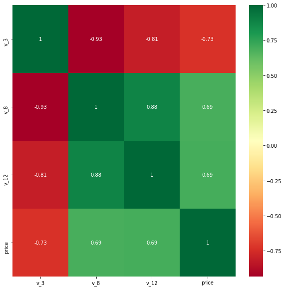
选择特征字段中与标签强相关的3个字段，绘制其与标签的分布关系图

threshold = 0.63

corrmat = data_train.corr()
top_corr_features = corrmat.index[abs(corrmat['price'])>threshold]
plt.figure(figsize = (10,10))
g = sns.heatmap(data_train[top_corr_features].corr(),
               annot = True,
               cmap = 'RdYlGn')

​

​

任务3：对标签进行数据分析，并使用log进行转换

使用Pandas对标签字段进行数据分析

预测值分布

Train_data['price']

0         1850
1         3600
2         6222
3         2400
4         5200
          ... 
149995    5900
149996    9500
149997    7500
149998    4999
149999    4700
Name: price, Length: 150000, dtype: int64

Train_data['price'].value_counts()

500      2337
1500     2158
1200     1922
1000     1850
2500     1821
         ... 
9395        1
81900       1
16699       1
11998       1
14780       1
Name: price, Length: 3763, dtype: int64

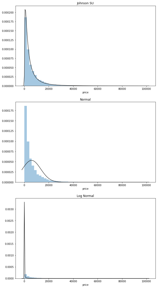
查看总体分布

distplot绘图函数作用详解：https://www.cnblogs.com/gczr/p/10354491.html#:~:text=displot ()会默认给出一个它认为比较好的组数，但是尝试不同的组数可能会揭示出数据不同的特征。 sns.displot（x%2Cbins%3D20%2Ckde%3DFalse%2Crug%3DTrue） 当绘制直方图时，最重要的参数是 bin 以及,vertical ，以确定直方图的组数和放置位置 sns.distplot (x%2C bins%3D20%2C kde%3DFalse%2C rug%3DTrue)%3B

y = Train_data['price']
plt.figure(figsize = (10,20))
ax = plt.subplot(3,1,1)
plt.title('Johnson SU')
sns.distplot(y,kde=False,fit = stats.johnsonsu)
ax = plt.subplot(3,1,2)
plt.title('Normal')
sns.distplot(y,kde=False,fit = stats.norm)
ax = plt.subplot(3,1,3)
plt.title('Log Normal')
sns.distplot(y,kde=False,fit = stats.lognorm)

<AxesSubplot:title={'center':'Log Normal'}, xlabel='price'>

​

​

使用log对标签字段进行转换

Train_data['price'] = np.log(Train_data['price'])

Train_data['price']

0         7.522941
1         8.188689
2         8.735847
3         7.783224
4         8.556414
            ...   
149995    8.682708
149996    9.159047
149997    8.922658
149998    8.516993
149999    8.455318
Name: price, Length: 150000, dtype: float64