经典网络层模型
AlexNet
模型介绍:
Alex Krizhevsky等人在2012年提出了AlexNe 并应用在大尺寸图片数据集ImageNet上,获得了2012年ImageNet比赛冠军。
AlexNet在LeNet的基础上加深了网络的结构,学习更丰富更高维的图像特征。AlexNet的特点:
- 更深的网络结构
- 使用层叠的卷积层,即卷积层+卷积层+池化层来提取图像的特征
- 使用Dropout抑制过拟合
- 使用数据增强Data Augmentation抑制过拟合
- 使用Relu替换之前的sigmoid的作为激活函数
- 多GPU训练
网络层大致结构:
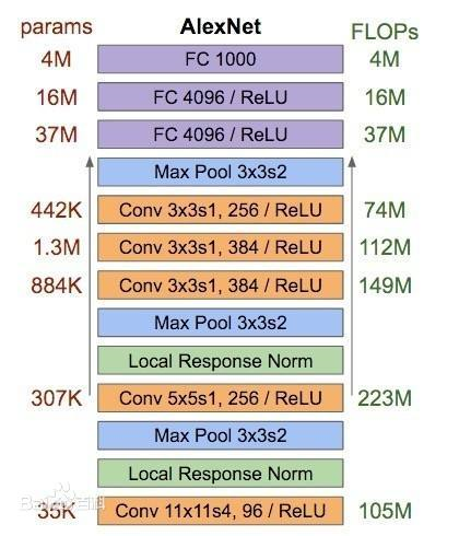
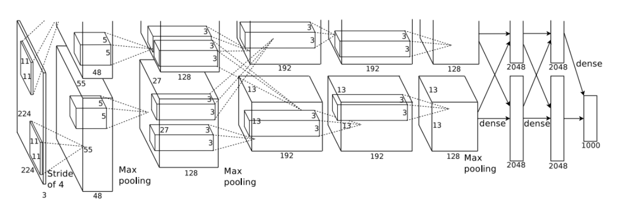
论文中的网络结构:
pytorch实现代码:
class AlexNet(nn.Module):

    def __init__(self, num_classes=1000):
        super(AlexNet, self).__init__()
        self.features = nn.Sequential(
            nn.Conv2d(3, 64, kernel_size=11, stride=4, padding=2),
            nn.ReLU(inplace=True),
            nn.MaxPool2d(kernel_size=3, stride=2),
            nn.Conv2d(64, 192, kernel_size=5, padding=2),
            nn.ReLU(inplace=True),
            nn.MaxPool2d(kernel_size=3, stride=2),
            nn.Conv2d(192, 384, kernel_size=3, padding=1),
            nn.ReLU(inplace=True),
            nn.Conv2d(384, 256, kernel_size=3, padding=1),
            nn.ReLU(inplace=True),
            nn.Conv2d(256, 256, kernel_size=3, padding=1),
            nn.ReLU(inplace=True),
            nn.MaxPool2d(kernel_size=3, stride=2),
        )
        self.avgpool = nn.AdaptiveAvgPool2d((6, 6))
        self.classifier = nn.Sequential(
            nn.Dropout(),
            nn.Linear(256 * 6 * 6, 4096),
            nn.ReLU(inplace=True),
            nn.Dropout(),
            nn.Linear(4096, 4096),
            nn.ReLU(inplace=True),
            nn.Linear(4096, num_classes),
        )

    def forward(self, x):
        x = self.features(x)
        x = self.avgpool(x)
        x = torch.flatten(x, 1)
        x = self.classifier(x)
        return x
ResNet
模型介绍:
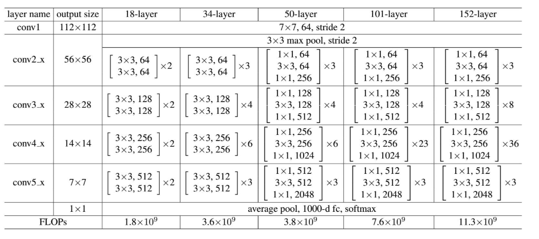
Residual Network,简称 ResNet(残差网络),是MSRA 何凯明团队设计的一种网络架构,在2015年的ILSVRC 和 COCO 上拿到了多项冠军,其发表的论文Deep Residual Learning for Image Recognition, 是 CVPR 2016的最佳论文。残差网络的特点是容易优化,并且能够通过增加相当的深度来提高准确率。其内部的残差块使用了跳跃连接,缓解了在深度神经网络中增加深度带来的梯度消失问题 。
内部残差块结构:

网络层大致结构:
pytorch实现代码:
class ResNet(nn.Module):

    def __init__(self, block, layers, num_classes=1000, zero_init_residual=False,
                 groups=1, width_per_group=64, replace_stride_with_dilation=None,
                 norm_layer=None):
        super(ResNet, self).__init__()
        if norm_layer is None:
            norm_layer = nn.BatchNorm2d
        self._norm_layer = norm_layer

        self.inplanes = 64
        self.dilation = 1
        if replace_stride_with_dilation is None:
            # each element in the tuple indicates if we should replace
            # the 2x2 stride with a dilated convolution instead
            replace_stride_with_dilation = [False, False, False]
        if len(replace_stride_with_dilation) != 3:
            raise ValueError("replace_stride_with_dilation should be None "
                             "or a 3-element tuple, got {}".format(replace_stride_with_dilation))
        self.groups = groups
        self.base_width = width_per_group
        self.conv1 = nn.Conv2d(3, self.inplanes, kernel_size=7, stride=2, padding=3,
                               bias=False)
        self.bn1 = norm_layer(self.inplanes)
        self.relu = nn.ReLU(inplace=True)
        self.maxpool = nn.MaxPool2d(kernel_size=3, stride=2, padding=1)
        self.layer1 = self._make_layer(block, 64, layers[0])
        self.layer2 = self._make_layer(block, 128, layers[1], stride=2,
                                       dilate=replace_stride_with_dilation[0])
        self.layer3 = self._make_layer(block, 256, layers[2], stride=2,
                                       dilate=replace_stride_with_dilation[1])
        self.layer4 = self._make_layer(block, 512, layers[3], stride=2,
                                       dilate=replace_stride_with_dilation[2])
        self.avgpool = nn.AdaptiveAvgPool2d((1, 1))
        self.fc = nn.Linear(512 * block.expansion, num_classes)

        for m in self.modules():
            if isinstance(m, nn.Conv2d):
                nn.init.kaiming_normal_(m.weight, mode='fan_out', nonlinearity='relu')
            elif isinstance(m, (nn.BatchNorm2d, nn.GroupNorm)):
                nn.init.constant_(m.weight, 1)
                nn.init.constant_(m.bias, 0)

        # Zero-initialize the last BN in each residual branch,
        # so that the residual branch starts with zeros, and each residual block behaves like an identity.
        # This improves the model by 0.2~0.3% according to https://arxiv.org/abs/1706.02677
        if zero_init_residual:
            for m in self.modules():
                if isinstance(m, Bottleneck):
                    nn.init.constant_(m.bn3.weight, 0)
                elif isinstance(m, BasicBlock):
                    nn.init.constant_(m.bn2.weight, 0)

    def _make_layer(self, block, planes, blocks, stride=1, dilate=False):
        norm_layer = self._norm_layer
        downsample = None
        previous_dilation = self.dilation
        if dilate:
            self.dilation *= stride
            stride = 1
        if stride != 1 or self.inplanes != planes * block.expansion:
            downsample = nn.Sequential(
                conv1x1(self.inplanes, planes * block.expansion, stride),
                norm_layer(planes * block.expansion),
            )

        layers = []
        layers.append(block(self.inplanes, planes, stride, downsample, self.groups,
                            self.base_width, previous_dilation, norm_layer))
        self.inplanes = planes * block.expansion
        for _ in range(1, blocks):
            layers.append(block(self.inplanes, planes, groups=self.groups,
                                base_width=self.base_width, dilation=self.dilation,
                                norm_layer=norm_layer))

        return nn.Sequential(*layers)

    def _forward_impl(self, x):
        # See note [TorchScript super()]
        x = self.conv1(x)
        x = self.bn1(x)
        x = self.relu(x)
        x = self.maxpool(x)

        x = self.layer1(x)
        x = self.layer2(x)
        x = self.layer3(x)
        x = self.layer4(x)

        x = self.avgpool(x)
        x = torch.flatten(x, 1)
        x = self.fc(x)

        return x

    def forward(self, x):
        return self._forward_impl(x)
DenseNet
模型介绍:
DenseNet模型的基本思路与ResNet一致,但是它建立的是前面所有层与后面层的密集连接(dense connection),它的名称也是由此而来。DenseNet的另一大特色是通过特征在channel上的连接来实现特征重用(feature reuse)。这些特点让DenseNet在参数和计算成本更少的情形下实现比ResNet更优的性能,DenseNet也因此斩获CVPR 2017的最佳论文奖。
模型大致结构:
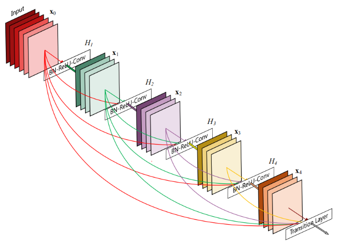
该架构与ResNet相比,在将特性传递到层之前,没有通过求和来组合特性,而是通过连接它们的方式来组合特性。因此第x层(输入层不算在内)将有x个输入,这些输入是之前所有层提取出的特征信息。
pytorch实现代码:
class _DenseLayer(nn.Module):
    def __init__(self, num_input_features, growth_rate, bn_size, drop_rate, memory_efficient=False):
        super(_DenseLayer, self).__init__()
        self.add_module('norm1', nn.BatchNorm2d(num_input_features)),
        self.add_module('relu1', nn.ReLU(inplace=True)),
        self.add_module('conv1', nn.Conv2d(num_input_features, bn_size *
                                           growth_rate, kernel_size=1, stride=1,
                                           bias=False)),
        self.add_module('norm2', nn.BatchNorm2d(bn_size * growth_rate)),
        self.add_module('relu2', nn.ReLU(inplace=True)),
        self.add_module('conv2', nn.Conv2d(bn_size * growth_rate, growth_rate,
                                           kernel_size=3, stride=1, padding=1,
                                           bias=False)),
        self.drop_rate = float(drop_rate)
        self.memory_efficient = memory_efficient

    def bn_function(self, inputs):
        # type: (List[Tensor]) -> Tensor
        concated_features = torch.cat(inputs, 1)
        bottleneck_output = self.conv1(self.relu1(self.norm1(concated_features)))  # noqa: T484
        return bottleneck_output

    # todo: rewrite when torchscript supports any
    def any_requires_grad(self, input):
        # type: (List[Tensor]) -> bool
        for tensor in input:
            if tensor.requires_grad:
                return True
        return False

    @torch.jit.unused  # noqa: T484
    def call_checkpoint_bottleneck(self, input):
        # type: (List[Tensor]) -> Tensor
        def closure(*inputs):
            return self.bn_function(*inputs)

        return cp.checkpoint(closure, input)

    @torch.jit._overload_method  # noqa: F811

    # torchscript does not yet support *args, so we overload method
    # allowing it to take either a List[Tensor] or single Tensor
    def forward(self, input):  # noqa: F811
        if isinstance(input, Tensor):
            prev_features = [input]
        else:
            prev_features = input

        if self.memory_efficient and self.any_requires_grad(prev_features):
            if torch.jit.is_scripting():
                raise Exception("Memory Efficient not supported in JIT")

            bottleneck_output = self.call_checkpoint_bottleneck(prev_features)
        else:
            bottleneck_output = self.bn_function(prev_features)

        new_features = self.conv2(self.relu2(self.norm2(bottleneck_output)))
        if self.drop_rate > 0:
            new_features = F.dropout(new_features, p=self.drop_rate,
                                     training=self.training)
        return new_features
GoogleNet
模型介绍:
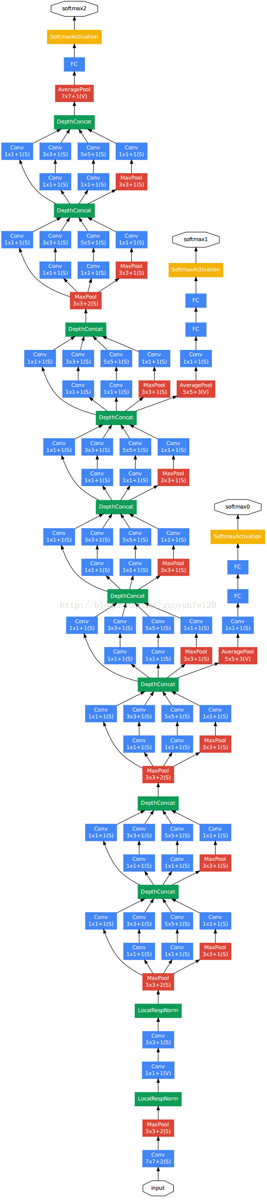
GoogLeNet是2014年Christian Szegedy提出的一种全新的深度学习结构,在这之前的AlexNet、VGG等结构都是通过增大网络的深度(层数)来获得更好的训练效果,但层数的增加会带来很多负作用,比如overfit、梯度消失、梯度爆炸等。inception的提出则从另一种角度来提升训练结果:能更高效的利用计算资源,在相同的计算量下能提取到更多的特征,从而提升训练结果。
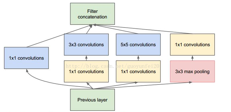
GoogleNet核心点共包括2个要素:
1)1x1卷积 2)多个尺寸上进行卷积再聚合
核心网络层大致结构:
模型大致结构:
pytorch实现代码:
class GoogLeNet(nn.Module):
    __constants__ = ['aux_logits', 'transform_input']

    def __init__(self, num_classes=1000, aux_logits=True, transform_input=False, init_weights=None,
                 blocks=None):
        super(GoogLeNet, self).__init__()
        if blocks is None:
            blocks = [BasicConv2d, Inception, InceptionAux]
        if init_weights is None:
            warnings.warn('The default weight initialization of GoogleNet will be changed in future releases of '
                          'torchvision. If you wish to keep the old behavior (which leads to long initialization times'
                          ' due to scipy/scipy#11299), please set init_weights=True.', FutureWarning)
            init_weights = True
        assert len(blocks) == 3
        conv_block = blocks[0]
        inception_block = blocks[1]
        inception_aux_block = blocks[2]

        self.aux_logits = aux_logits
        self.transform_input = transform_input

        self.conv1 = conv_block(3, 64, kernel_size=7, stride=2, padding=3)
        self.maxpool1 = nn.MaxPool2d(3, stride=2, ceil_mode=True)
        self.conv2 = conv_block(64, 64, kernel_size=1)
        self.conv3 = conv_block(64, 192, kernel_size=3, padding=1)
        self.maxpool2 = nn.MaxPool2d(3, stride=2, ceil_mode=True)

        self.inception3a = inception_block(192, 64, 96, 128, 16, 32, 32)
        self.inception3b = inception_block(256, 128, 128, 192, 32, 96, 64)
        self.maxpool3 = nn.MaxPool2d(3, stride=2, ceil_mode=True)

        self.inception4a = inception_block(480, 192, 96, 208, 16, 48, 64)
        self.inception4b = inception_block(512, 160, 112, 224, 24, 64, 64)
        self.inception4c = inception_block(512, 128, 128, 256, 24, 64, 64)
        self.inception4d = inception_block(512, 112, 144, 288, 32, 64, 64)
        self.inception4e = inception_block(528, 256, 160, 320, 32, 128, 128)
        self.maxpool4 = nn.MaxPool2d(2, stride=2, ceil_mode=True)

        self.inception5a = inception_block(832, 256, 160, 320, 32, 128, 128)
        self.inception5b = inception_block(832, 384, 192, 384, 48, 128, 128)

        if aux_logits:
            self.aux1 = inception_aux_block(512, num_classes)
            self.aux2 = inception_aux_block(528, num_classes)
        else:
            self.aux1 = None
            self.aux2 = None

        self.avgpool = nn.AdaptiveAvgPool2d((1, 1))
        self.dropout = nn.Dropout(0.2)
        self.fc = nn.Linear(1024, num_classes)

        if init_weights:
            self._initialize_weights()

    def _initialize_weights(self):
        for m in self.modules():
            if isinstance(m, nn.Conv2d) or isinstance(m, nn.Linear):
                import scipy.stats as stats
                X = stats.truncnorm(-2, 2, scale=0.01)
                values = torch.as_tensor(X.rvs(m.weight.numel()), dtype=m.weight.dtype)
                values = values.view(m.weight.size())
                with torch.no_grad():
                    m.weight.copy_(values)
            elif isinstance(m, nn.BatchNorm2d):
                nn.init.constant_(m.weight, 1)
                nn.init.constant_(m.bias, 0)

    def _transform_input(self, x):
        # type: (Tensor) -> Tensor
        if self.transform_input:
            x_ch0 = torch.unsqueeze(x[:, 0], 1) * (0.229 / 0.5) + (0.485 - 0.5) / 0.5
            x_ch1 = torch.unsqueeze(x[:, 1], 1) * (0.224 / 0.5) + (0.456 - 0.5) / 0.5
            x_ch2 = torch.unsqueeze(x[:, 2], 1) * (0.225 / 0.5) + (0.406 - 0.5) / 0.5
            x = torch.cat((x_ch0, x_ch1, x_ch2), 1)
        return x

    def _forward(self, x):
        # type: (Tensor) -> Tuple[Tensor, Optional[Tensor], Optional[Tensor]]
        # N x 3 x 224 x 224
        x = self.conv1(x)
        # N x 64 x 112 x 112
        x = self.maxpool1(x)
        # N x 64 x 56 x 56
        x = self.conv2(x)
        # N x 64 x 56 x 56
        x = self.conv3(x)
        # N x 192 x 56 x 56
        x = self.maxpool2(x)

        # N x 192 x 28 x 28
        x = self.inception3a(x)
        # N x 256 x 28 x 28
        x = self.inception3b(x)
        # N x 480 x 28 x 28
        x = self.maxpool3(x)
        # N x 480 x 14 x 14
        x = self.inception4a(x)
        # N x 512 x 14 x 14
        aux1 = torch.jit.annotate(Optional[Tensor], None)
        if self.aux1 is not None:
            if self.training:
                aux1 = self.aux1(x)

        x = self.inception4b(x)
        # N x 512 x 14 x 14
        x = self.inception4c(x)
        # N x 512 x 14 x 14
        x = self.inception4d(x)
        # N x 528 x 14 x 14
        aux2 = torch.jit.annotate(Optional[Tensor], None)
        if self.aux2 is not None:
            if self.training:
                aux2 = self.aux2(x)

        x = self.inception4e(x)
        # N x 832 x 14 x 14
        x = self.maxpool4(x)
        # N x 832 x 7 x 7
        x = self.inception5a(x)
        # N x 832 x 7 x 7
        x = self.inception5b(x)
        # N x 1024 x 7 x 7

        x = self.avgpool(x)
        # N x 1024 x 1 x 1
        x = torch.flatten(x, 1)
        # N x 1024
        x = self.dropout(x)
        x = self.fc(x)
        # N x 1000 (num_classes)
        return x, aux2, aux1

    @torch.jit.unused
    def eager_outputs(self, x, aux2, aux1):
        # type: (Tensor, Optional[Tensor], Optional[Tensor]) -> GoogLeNetOutputs
        if self.training and self.aux_logits:
            return _GoogLeNetOutputs(x, aux2, aux1)
        else:
            return x

    def forward(self, x):
        # type: (Tensor) -> GoogLeNetOutputs
        x = self._transform_input(x)
        x, aux1, aux2 = self._forward(x)
        aux_defined = self.training and self.aux_logits
        if torch.jit.is_scripting():
            if not aux_defined:
                warnings.warn("Scripted GoogleNet always returns GoogleNetOutputs Tuple")
            return GoogLeNetOutputs(x, aux2, aux1)
        else:
            return self.eager_outputs(x, aux2, aux1)
VggNet
模型介绍:
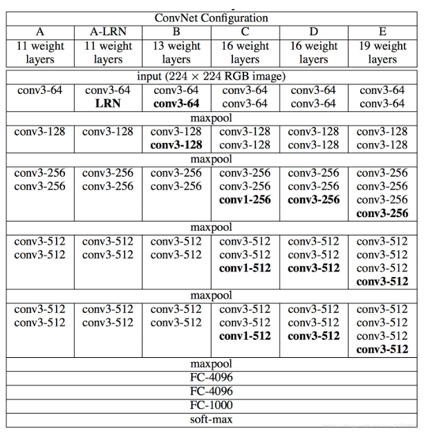
VGGNet由牛津大学计算机视觉组合和Google DeepMind公司研究员一起研发的深度卷积神经网络。它探索了卷积神经网络的深度和其性能之间的关系,通过反复的堆叠3x3的小型卷积核和2x2的最大池化层,成功的构建了16~19层深的卷积神经网络。VGGNet获得了ILSVRC 2014年比赛的亚军和定位项目的冠军,在top5上的错误率为7.5%。目前为止,VGGNet依然被用来提取图像的特征。
GGNet全部使用3x3的卷积核和2x2的池化核,通过不断加深网络结构来提升性能。网络层数的增长并不会带来参数量上的爆炸,因为参数量主要集中在最后三个全连接层中。同时,两个3x3卷积层的串联相当于1个5x5的卷积层,3个3x3的卷积层串联相当于1个7x7的卷积层,即3个3x3卷积层的感受野大小相当于1个7x7的卷积层。但是3个3x3的卷积层参数量只有7x7的一半左右,同时前者可以有3个非线性操作,而后者只有1个非线性操作,这样使得前者对于特征的学习能力更强。
模型大致结构:
pytorch生成代码:
class VGG(nn.Module):

    def __init__(self, features, num_classes=1000, init_weights=True):
        super(VGG, self).__init__()
        self.features = features
        self.avgpool = nn.AdaptiveAvgPool2d((7, 7))
        self.classifier = nn.Sequential(
            nn.Linear(512 * 7 * 7, 4096),
            nn.ReLU(True),
            nn.Dropout(),
            nn.Linear(4096, 4096),
            nn.ReLU(True),
            nn.Dropout(),
            nn.Linear(4096, num_classes),
        )
        if init_weights:
            self._initialize_weights()

    def forward(self, x):
        x = self.features(x)
        x = self.avgpool(x)
        x = torch.flatten(x, 1)
        x = self.classifier(x)
        return x
ShuffleNet
模型介绍
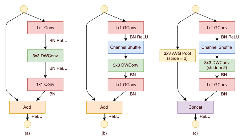
ShuffleNet是专门为计算能力非常有限的移动设备(例如,10-150 MFLOPs)而设计的。该结构利用分组逐点卷积(pointwise group convolution)和通道重排(channel shuffle)两种新的运算方法,在保证计算精度的同时,大大降低了计算成本。ImageNet分类和MS COCO目标检测实验表明,在40 MFLOPs计算预算下,ShuffleNet的性能优于其他结构,例如,在ImageNet分类任务上,与最近的MobileNet相比,top-1错误率(绝对7.8%)更低。在基于arm的移动设备上,ShuffleNet比AlexNet实现了约13倍的实际加速,同时保持了相当的准确性。
ShuffleNet单元结构:
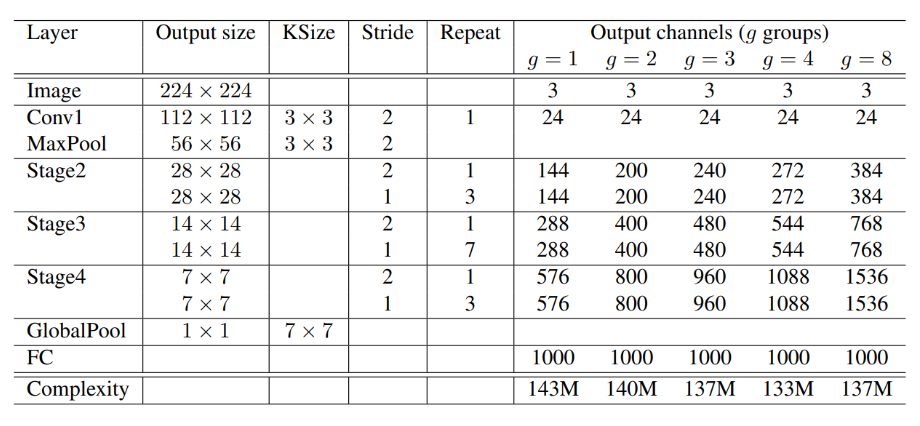
模型大致结构:
pytorch生成代码:
class ShuffleNetV2(nn.Module):
    def __init__(self, stages_repeats, stages_out_channels, num_classes=1000, inverted_residual=InvertedResidual):
        super(ShuffleNetV2, self).__init__()

        if len(stages_repeats) != 3:
            raise ValueError('expected stages_repeats as list of 3 positive ints')
        if len(stages_out_channels) != 5:
            raise ValueError('expected stages_out_channels as list of 5 positive ints')
        self._stage_out_channels = stages_out_channels

        input_channels = 3
        output_channels = self._stage_out_channels[0]
        self.conv1 = nn.Sequential(
            nn.Conv2d(input_channels, output_channels, 3, 2, 1, bias=False),
            nn.BatchNorm2d(output_channels),
            nn.ReLU(inplace=True),
        )
        input_channels = output_channels

        self.maxpool = nn.MaxPool2d(kernel_size=3, stride=2, padding=1)

        stage_names = ['stage{}'.format(i) for i in [2, 3, 4]]
        for name, repeats, output_channels in zip(
                stage_names, stages_repeats, self._stage_out_channels[1:]):
            seq = [inverted_residual(input_channels, output_channels, 2)]
            for i in range(repeats - 1):
                seq.append(inverted_residual(output_channels, output_channels, 1))
            setattr(self, name, nn.Sequential(*seq))
            input_channels = output_channels

        output_channels = self._stage_out_channels[-1]
        self.conv5 = nn.Sequential(
            nn.Conv2d(input_channels, output_channels, 1, 1, 0, bias=False),
            nn.BatchNorm2d(output_channels),
            nn.ReLU(inplace=True),
        )

        self.fc = nn.Linear(output_channels, num_classes)

    def _forward_impl(self, x):
        # See note [TorchScript super()]
        x = self.conv1(x)
        x = self.maxpool(x)
        x = self.stage2(x)
        x = self.stage3(x)
        x = self.stage4(x)
        x = self.conv5(x)
        x = x.mean([2, 3])  # globalpool
        x = self.fc(x)
        return x

    def forward(self, x):
        return self._forward_impl(x)
教学模型
mnist预测模型
mnist数据集介绍
MNIST 数据集来自美国国家标准与技术研究所, National Institute of Standards and Technology (NIST). 训练集 (training set) 由来自 250 个不同人手写的数字构成, 其中 50% 是高中学生, 50% 来自人口普查局 (the Census Bureau) 的工作人员. 测试集(test set) 也是同样比例的手写数字数据。
mnist_model1
以下介绍对于mnist数据集的一个简单的预测模型,只使用了激活层和全连接层,具体结构如下图所示:
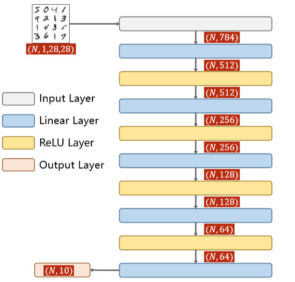
如上图所示,本模型结构较为简单,将全连接层串联在一起,并在每个全连接层之间使用Relu进行激活。
生成的具体函数如下图所示:
class Net(torch.nn.Module):
def __init__(self):
super(Net, self).__init__()
self.l1 = torch.nn.Linear(784, 512)
self.l2 = torch.nn.Linear(512, 256)
self.l3 = torch.nn.Linear(256, 128)
self.l4 = torch.nn.Linear(128, 64)
self.l5 = torch.nn.Linear(64, 10)
def forward(self, x):
x = x.view(-1, 784)
x = F.relu(self.l1(x))
x = F.relu(self.l2(x))
x = F.relu(self.l3(x))
x = F.relu(self.l4(x))
return self.l5(x)
本模型对应的损失函数为CrossEntropyLoss(交叉商损失函数),具体计算步骤可参见下图内容:
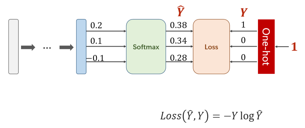
如上图所示,CrossEntropyLoss将softmax层与NLLLOSS函数进行拼接,最后输出的向量中保证只有一个分量的值为1,其他分量的值为0。mnist数据集模型要求对于数字0-9图片进行分类并且识别,因此CrossEntropyLoss具有非常好的适用性。
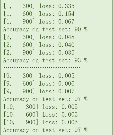
虽然结构较为简单,但是mnist_model1具有非常高的准确性,能够达到97%的准确率。具体结果如下图所示:
mnist_model2
模型链接:
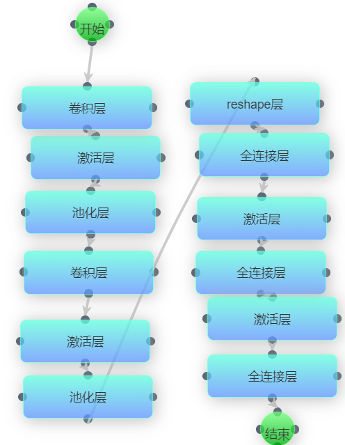
mnist_model2在mnist_model1的基础上增加了卷积层以及池化层,能够哦更好地对图片进行分类识别,模型具体结构如下图所示:
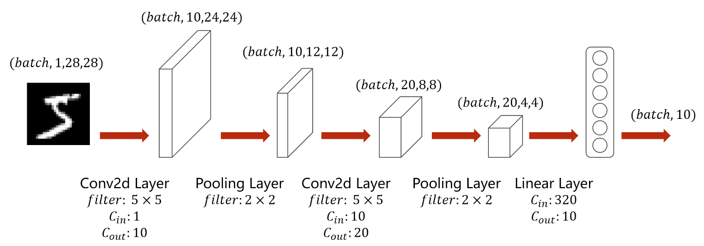
mnist_model2对输入数据进行了两次卷积以及池化,同时在池化后对数据内容进行激活。最终经过全连接层后进行结果输出。
生成的具体函数代码如下图所示:
class Net(torch.nn.Module):
def __init__(self):
super(Net, self).__init__()
self.conv1 = torch.nn.Conv2d(1, 10, kernel_size=5)
self.conv2 = torch.nn.Conv2d(10, 20, kernel_size=5)
self.pooling = torch.nn.MaxPool2d(2)
self.fc = torch.nn.Linear(320, 10)

def forward(self, x):
batch_size = x.size(0)
x = F.relu(self.pooling(self.conv1(x)))
x = F.relu(self.pooling(self.conv2(x)))
x = x.view(batch_size, -1)
x = self.fc(x)
return x
本模型使用的损失函数与mnist_model1相同,不再赘述。
mnist_model2由于采用了更适合进行图像识别的卷积层,因此对于图像识别的准确率更高,具体数值如下图所示:

由上图可见,mnist_model2的准确率达到了98%。虽然相较于mnist_model1只高出了1%,但从比例上来查看相较于mnist_model1的出错率降低了1/3,在进行较大规模图像识别时本模型具有较高的优势。
cifar10预测模型
cifar10数据集介绍
CIFAR-10 是由 Hinton 的学生 Alex Krizhevsky 和 Ilya Sutskever 整理的一个用于识别普适物体的小型数据集。一共包含 10 个类别的 RGB 彩色图 片:飞机( a叩lane )、汽车( automobile )、鸟类( bird )、猫( cat )、鹿( deer )、狗( dog )、蛙类( frog )、马( horse )、船( ship )和卡车( truck )。图片的尺寸为 32×32 ,数据集中一共有 50000 张训练圄片和 10000 张测试图片。 CIFAR-10 的图片样例如图所示。
下面这幅图就是列举了10各类,每一类展示了随机的10张图片:
与 MNIST 数据集中目比, CIFAR-10 具有以下不同点:
• CIFAR-10 是 3 通道的彩色 RGB 图像,而 MNIST 是灰度图像。
• CIFAR-10 的图片尺寸为 32×32, 而 MNIST 的图片尺寸为 28×28,比 MNIST 稍大。
• 相比于手写字符, CIFAR-10 含有的是现实世界中真实的物体,不仅噪声很大,而且物体的比例、 特征都不尽相同,这为识别带来很大困难。 直接的线性模型如 Softmax 在 CIFAR-10 上表现得很差。
cifar10_model1
该模型参照了pytorch官网对于cifar10数据集的教程。本模型结构较为简单,只对数据进行了卷积、池化以及全连接操作。模型结构如下图所示:
这种结构的网络效果其实不好,因为全连接层传递效率较低,同时会干扰到卷积层提取出的局部特征,并且也没有用到BatchNorm和Dropout来防止过拟合的问题。而cifar10数据集结构较为复杂,因此cifar10_model1精度较差。
生成具体函数代码如下图所示:
class Net(nn.Module):
    def __init__(self):
       super(Net, self).__init__()
        self.conv1 = nn.Conv2d(3, 6, 5)
        self.pool = nn.MaxPool2d(2, 2)
        self.conv2 = nn.Conv2d(6, 16, 5)
        self.fc1 = nn.Linear(16 * 5 * 5, 120)
        self.fc2 = nn.Linear(120, 84)
        self.fc3 = nn.Linear(84, 10)

def forward(self, x):
    x = self.pool(F.relu(self.conv1(x)))
    x = self.pool(F.relu(self.conv2(x)))
    x = x.view(-1, 16 * 5 * 5)
    x = F.relu(self.fc1(x))
    x = F.relu(self.fc2(x))
    x = self.fc3(x)
由于数据集与mnist同为图像分类识别数据集,因此损失函数和优化器与mnist数据集中的保持一致,如下图所示:
criterion = nn.CrossEntropyLoss()

optimizer = optim.Adam(net.parameters(), lr=0.001)
模型最终的准确率并不高,能够达到 %,如下图所示:
cifar10_model2
在cifar10_model1的基础上,cifar10_model2增加了batchnorm层以及dropout层防止过拟合操作。具体模型结构如下图所示:
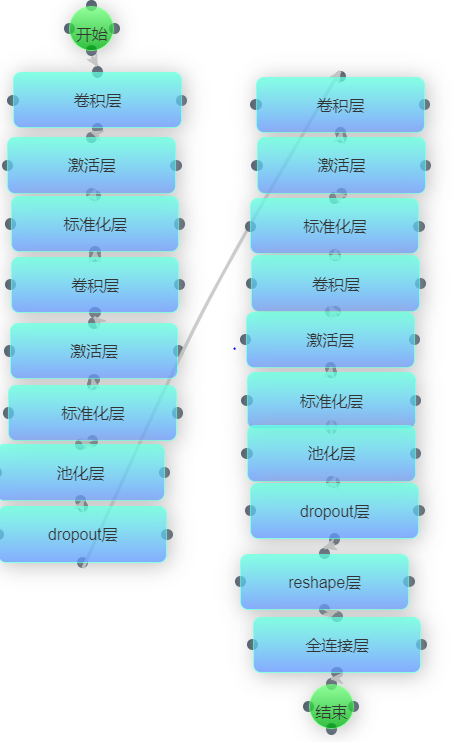
对于cifar10这样结构较为复杂的数据集,cifar10_model2能够去除数据中的噪声同时有效防止过拟合。
生成的代码如下所示:
class Net(nn.Module):
    def __init__(self):
        super(Net, self).__init__()
        self.conv1 = nn.Conv2d(3, 64, 3, padding = 1)
        self.conv2 = nn.Conv2d(64, 64, 3, padding = 1)
        self.conv3 = nn.Conv2d(64, 128, 3, padding = 1)
        self.conv4 = nn.Conv2d(128, 128, 3, padding = 1)
        self.conv5 = nn.Conv2d(128, 256, 3, padding = 1)
        self.conv6 = nn.Conv2d(256, 256, 3, padding = 1)
        self.maxpool = nn.MaxPool2d(2, 2)
        self.avgpool = nn.AvgPool2d(2, 2)
        self.globalavgpool = nn.AvgPool2d(8, 8)
        self.bn1 = nn.BatchNorm2d(64)
        self.bn2 = nn.BatchNorm2d(128)
        self.bn3 = nn.BatchNorm2d(256)
        self.dropout50 = nn.Dropout(0.5)
        self.dropout10 = nn.Dropout(0.1)
        self.fc = nn.Linear(256, 10)

def forward(self, x):
    x = self.bn1(F.relu(self.conv1(x)))
    x = self.bn1(F.relu(self.conv2(x)))
    x = self.maxpool(x)
    x = self.dropout10(x)
    x = self.bn2(F.relu(self.conv3(x)))
    x = self.bn2(F.relu(self.conv4(x)))
    x = self.avgpool(x)
    x = self.dropout10(x)
    x = self.bn3(F.relu(self.conv5(x)))
    x = self.bn3(F.relu(self.conv6(x)))
    x = self.globalavgpool(x)
    x = self.dropout50(x)
    x = x.view(x.size(0), -1)
    x = self.fc(x)
由于数据集与mnist同为图像分类识别数据集,因此损失函数和优化器与mnist数据集中的保持一致,如下图所示:
criterion = nn.CrossEntropyLoss()

optimizer = optim.Adam(net.parameters(), lr=0.001)
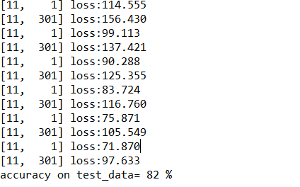
cifar10_model2在batch_size=100的条件下训练10个epoch之后,测试集正确率大概在80%左右。对于cifar10这样的数据集准确率已经较高了,结果如下图所示: