中文数据集THUCNews:https://pan.baidu.com/s/1hugrfRu 密码:qfud
参考:https://blog.csdn.net/SMith7412/article/details/88087819
参考:https://blog.csdn.net/u011439796/article/details/77692621
1.THUCNews数据集下载和探索
基于清华THUCNews新闻文本分类数据集的一个子集,预处理部分对其中的10个类别的相关文本数据进行处理。
类别: ['体育', '财经', '房产', '家居', '教育', '科技', '时尚', '时政', '游戏', '娱乐']
cnews.train.txt: 训练集(50000条)
预处理文件为cnews/cnews_loader.py
按照逻辑顺序定义函数:
open_file:打开文件
read_file:读取文件,并返回 contents,labels
build_vocab: 构建词汇表,并且保存在本地txt中,避免每次都进行重复work.
read_category:读取类别,将类别转化为id,{类别:id}
read_vocab:读取build好的词汇表,{词:id}
process_file:将文件转化为id表示存到data_id和label_id中,并且用keras的pad函数进行填充为指定大小,返回array
batch_iter:根据batch的大小对数据进行按批次生成
相关代码:
 1 import sys
 2 from collections import Counter
 3 import numpy as np
 4 import tensorflow.contrib.keras as kr
 5
 6 def build_vocab(train_dir,vocab_dir,vocab_size=5000):
 7     """根据训练集构建词汇表,存储"""
 8     data_train,_ = read_file(train_dir)
 9     all_data = []
10     for content in data_train:#['马', '晓', '旭', '意', '外', '受', '伤'.....]
11         all_data.extend(content)#['马', '晓', '旭', '意', '外', '受', '伤'.....]所有内容变成单个字
12     counter = Counter(all_data)#计算每个字出现的次数,返回Counter({',': 1871208, '的': 1414310, '。': 822140, '一': 443181, ...})
13     count_pairs = counter.most_common(vocab_size - 1)#返回一个list [(',', 1871208), ('的', 1414310), ('。', 822140), ('一', 443181)....]
14     words,_ = list(zip(*count_pairs))
15
16     words=['<PAD>']+list(words)
17     open_file(vocab_dir,mode='w').write('
'.join(words)+'
')
18
19
20 def read_file(filename):
21     """读取文件数据"""
22     contents,labels=[],[]
23     with open_file(filename) as f:
24         for line in f:
25             try:
26                 label,content = line.strip().stplit('	')#label = '体育' content ='马晓旭意外受伤。。。。。'
27                 if content:
28                     contents.append(list(content))#list('1234')->> ['1','2','3','4']
29                     labels.append(label)
30             except:
31                 pass
32     return contents,labels
33
34 def open_file(filename,mode='r'):
35     return open(filename,mode,encoding='utf8',errors='ignore')
36 def read_category():
37     categories=['体育', '财经', '房产', '家居', '教育', '科技', '时尚', '时政', '游戏', '娱乐']
38     cat_to_id = dict(zip(categories,range(len(categories))))
39     return categories,cat_to_id
40
41 def read_vocab(vocab_dir):
42     with open_file(vocab_dir) as fp:
43         words = [_.strip() for _ in fp.readlines()]
44     word_to_id = dict(zip(words,range(len(words))))
45     return words,word_to_id
46
47 def process_file(filename,word_to_id,cat_to_id,max_length=600):
48     """将文件转换为id表示"""
49     contents,labels = read_file(filename)
50     data_id,label_id=[],[]
51     for i in range(len(contents)):
52         data_id.append([word_to_id[x] for x in contents[i] if x in word_to_id]):
53         label_id.append(cat_to_id[labels[i]])
54     #用kears提供的pad_sequence 来将文本pad为固定长度
55     x_pad = kr.preprocessiong.sequence.pad_sequences(data_id,max_length)
56     y_pad = kr.utils.to_categorical(label_id,num_classes=len(cat_to_id))#将标签转换为one_hot表示
57
58 def batch_iter(x,y,batch_size=64):
59     """生成批次数据"""
60     data_len = len(x)
61     num_batch = int((data_len - 1) / batch_size) + 1
62     indices = np.random.permutation(np.arange(data_len))
63     x_shuffle = x[indices]
64     y_shuffle = y[indices]
65
66     for i in range(num_batch):
67         start_id = i * batch_size
68         end_id = min((i+1)*batch_size,data_len)
69         yield x_shuffle[start_id:end_id],y_shuffle[start_id:end_id]#yield函数类似于return但是返回的是generator只不过是下次执行从其下一条语句开始。
70
2.IMDB数据集探索
参考TensorFlow官方教程:https://tensorflow.google.cn/tutorials/keras/basic_text_classification
load_data时,numpy1.16.3会报错,最好改成1.16.1 pip3 install numpy==1.16.1
官方已经对数据集进行了处理:包含来自互联网电影数据库的 50000 条影评文本。我们将这些影评拆分为训练集(25000 条影评)和测试集(25000 条影评)。训练集和测试集之间达成了平衡,意味着它们包含相同数量的正面和负面影评。将影评(字词序列)转换为整数序列,其中每个整数表示字典中的一个特定字词。
1 import tensorflow as tf
2 from tensorflow import keras
3
4 import numpy as np
5 print(tf.__version__)
》》》1.13.1
1 imdb = keras.datasets.imdb#nums_words=10000,会保留训练数据中出现频次在前10000位的字词,确保数据规模不太大,罕见字将被抛弃
2 (train_data, train_labels), (test_data, test_labels) = imdb.load_data(path='E:/soft/notebooks/nlp/imdb.npz',num_words=10000)
每个样本为一个整数数组表示影评中的字词,每个标签为0(负面影评)或1(正面影评)
1 print('Training entries:{},labels:{}'.format(len(train_data),len(train_labels)))
》》》Training entries:25000,labels:25000
我们来看一下第一条影评
1 print(train_data[0])
[1, 14, 22, 16, 43, 530, 973, 1622, 1385, 65, 458, 4468, 66, 3941, 4, 173, 36, 256, 5, 25, 100, 43, 838, 112, 50, 670, 2, 9, 35, 480, 284, 5, 150, 4, 172, 112, 167, 2, 336, 385, 39, 4, 172, 4536, 1111, 17, 546, 38, 13, 447, 4, 192, 50, 16, 6, 147, 2025, 19, 14, 22, 4, 1920, 4613, 469, 4, 22, 71, 87, 12, 16, 43, 530, 38, 76, 15, 13, 1247, 4, 22, 17, 515, 17, 12, 16, 626, 18, 2, 5, 62, 386, 12, 8, 316, 8, 106, 5, 4, 2223, 5244, 16, 480, 66, 3785, 33, 4, 130, 12, 16, 38, 619, 5, 25, 124, 51, 36, 135, 48, 25, 1415, 33, 6, 22, 12, 215, 28, 77, 52, 5, 14, 407, 16, 82, 2, 8, 4, 107, 117, 5952, 15, 256, 4, 2, 7, 3766, 5, 723, 36, 71, 43, 530, 476, 26, 400, 317, 46, 7, 4, 2, 1029, 13, 104, 88, 4, 381, 15, 297, 98, 32, 2071, 56, 26, 141, 6, 194, 7486, 18, 4, 226, 22, 21, 134, 476, 26, 480, 5, 144, 30, 5535, 18, 51, 36, 28, 224, 92, 25, 104, 4, 226, 65, 16, 38, 1334, 88, 12, 16, 283, 5, 16, 4472, 113, 103, 32, 15, 16, 5345, 19, 178, 32]
影评长度可能会有所不同,神经网络要求输入必须具有相同长度
len(train_data[0]),len(train_data[1])
>>>(218, 189)
下面来看一下如何把整数转换为字词,通过创建辅助函数来查询整数到字符映射的字典对象
word_index = imdb.get_word_index()

word_index = {k:(v+3) for k,v in word_index.items()}
word_index["<PAD>"] = 0
word_index["<START>"] = 1
word_index["<UNK>"]=2
word_index["<UNUSED>"] =3
reverse_word_index = dict([(value,key) for (key,value) in word_index.items()])
def decode_review(text):
    return ' '.join([reverse_word_index.get(i,'?') for i in text])
下面使用decode_review函数显示第一条影评的文本
decode_review(train_data[0])
>>>>
"<START> this film was just brilliant casting location scenery story direction everyone's really suited the part they played and you could just imagine being there robert <UNK> is an amazing actor and now the same being director <UNK> father came from the same scottish island as myself so i loved the fact there was a real connection with this film the witty remarks throughout the film were great it was just brilliant so much that i bought the film as soon as it was released for <UNK> and would recommend it to everyone to watch and the fly fishing was amazing really cried at the end it was so sad and you know what they say if you cry at a film it must have been good and this definitely was also <UNK> to the two little boy's that played the <UNK> of norman and paul they were just brilliant children are often left out of the <UNK> list i think because the stars that play them all grown up are such a big profile for the whole film but these children are amazing and should be praised for what they have done don't you think the whole story was so lovely because it was true and was someone's life after all that was shared with us all"
准备数据
影评必须转换为张量,然后才能馈送到神经网络中,我们可以通过下述方法进行转换
·对数组进行独热编码,将它们转换为由 0 和 1 构成的向量。然后,将它作为网络的第一层,一个可以处理浮点向量数据的密集层。不过,这种方法会占用大量内存,需要一个大小为 num_words * num_reviews 的矩阵。
·或者可以填充数组,使他们都具有相同的长度,然后创建一个形状为max_length * num_reviews的整数张量。我们可以使用一个能够处理这种形状的嵌入层作为网络中的第一层。
我们来使用第二种方法进行长度标准化
1 train_data = keras.preprocessing.sequence.pad_sequences(train_data,
2                                                        value=word_index['<PAD>'],
3                                                        padding='post',
4                                                        maxlen=256)
5 test_data = keras.preprocessing.sequence.pad_sequences(test_data,
6                                                       value=word_index['<PAD>'],
7                                                       maxlen=256)
len(train_data[0]),len(train_data[1])
(256,256)
看一下填充后的第一条影评
[   1   14   22   16   43  530  973 1622 1385   65  458 4468   66 3941
    4  173   36  256    5   25  100   43  838  112   50  670    2    9
   35  480  284    5  150    4  172  112  167    2  336  385   39    4
  172 4536 1111   17  546   38   13  447    4  192   50   16    6  147
 2025   19   14   22    4 1920 4613  469    4   22   71   87   12   16
   43  530   38   76   15   13 1247    4   22   17  515   17   12   16
  626   18    2    5   62  386   12    8  316    8  106    5    4 2223
 5244   16  480   66 3785   33    4  130   12   16   38  619    5   25
  124   51   36  135   48   25 1415   33    6   22   12  215   28   77
   52    5   14  407   16   82    2    8    4  107  117 5952   15  256
    4    2    7 3766    5  723   36   71   43  530  476   26  400  317
   46    7    4    2 1029   13  104   88    4  381   15  297   98   32
 2071   56   26  141    6  194 7486   18    4  226   22   21  134  476
   26  480    5  144   30 5535   18   51   36   28  224   92   25  104
    4  226   65   16   38 1334   88   12   16  283    5   16 4472  113
  103   32   15   16 5345   19  178   32    0    0    0    0    0    0
    0    0    0    0    0    0    0    0    0    0    0    0    0    0
    0    0    0    0    0    0    0    0    0    0    0    0    0    0
    0    0    0    0]
构建模型
神经网络是通过堆叠层创建而成,要做出两个架构方面的主要决策
·要在模型中使用多少层
·要针对每个层使用多少个隐藏单元
在本示例中,输入数据有字词-索引数组构成,要预测的标签为0或1.为此我们建立以下模型
1 vocab_size = 10000
2
3 model = keras.Sequential()
4 model.add(keras.layers.Embedding(vocab_size,16))#Embedding层,此层会在整数编码的词汇表中查找每个词-索引的嵌入向量,模型在训练时会学习这些向量,这些向量回想
5 model.add(keras.layers.GlobalAveragePooling1D())
6 model.add(keras.layers.Dense(16,activation=tf.nn.relu))
7 model.add(keras.layers.Dense(1,activation=tf.nn.sigmoid))
8
9 model.summary()
Instructions for updating:
Colocations handled automatically by placer.
_________________________________________________________________
Layer (type)                 Output Shape              Param #
=================================================================
embedding (Embedding)        (None, None, 16)          160000
_________________________________________________________________
global_average_pooling1d (Gl (None, 16)                0
_________________________________________________________________
dense (Dense)                (None, 16)                272
_________________________________________________________________
dense_1 (Dense)              (None, 1)                 17
=================================================================
Total params: 160,289
Trainable params: 160,289
Non-trainable params: 0
按顺序堆叠各个层以构建分类器:
- 第一层是
Embedding层。该层会在整数编码的词汇表中查找每个字词-索引的嵌入向量。模型在接受训练时会学习这些向量。这些向量会向输出数组添加一个维度。生成的维度为:(batch, sequence, embedding)。 - 接下来,一个
GlobalAveragePooling1D层通过对序列维度求平均值,针对每个样本返回一个长度固定的输出向量。这样,模型便能够以尽可能简单的方式处理各种长度的输入。 - 该长度固定的输出向量会传入一个全连接 (
Dense) 层(包含 16 个隐藏单元)。 - 最后一层与单个输出节点密集连接。应用
sigmoid激活函数后,结果是介于 0 到 1 之间的浮点值,表示概率或置信水平。
隐藏单元:
输入层和输出层之间的层被称为隐藏层,输出(单元,节点,或神经元)的数量是相应层的表示法空间的维度,换句话,该数值表示学习内部表示法时网络所允许的自由度。
模型层数越多,则网络可以学习更复杂的表示法,但是会消耗网络资源,也可能会过拟合(神经网络模型一般都会过拟合的)。
损失函数和优化器:
损失函数用的是binary_crossentropy,与mean_squared_error比较,binary_crossentropy更适合处理概率问题,它可测量概率分布之间的“差距”,在本例中为实际分布和预测之间的“差距”。
配置模型以使用优化器和损失函数:
model.compile(optimizer=tf.train.AdadeltaOptimizer(),
             loss='binary_crossentropy',
             metrics=['accuracy'])
创建验证集:
在训练时,我们要检查模型从未见过的数据的准确率,其实验证集的目的是调整超参数。不用测试集的目的是,我们的目标是仅使用训练数据开发和调整模型,然后仅使用一次测试数据评估准确率。
x_val = train_data[:10000]
partial_x_train = train_data[10000:]

y_val = train_labels[:10000]
partial_y_train = train_labels[10000:]
训练模型:
用每个含有512个样本的batch训练40个epoch,对x_train和y_train所有张量进行40次迭代。
Instructions for updating:
Use tf.cast instead.
Epoch 1/40
15000/15000 [==============================] - 2s 149us/sample - loss: 0.6931 - acc: 0.5033 - val_loss: 0.6932 - val_acc: 0.4956
Epoch 2/40
15000/15000 [==============================] - 1s 97us/sample - loss: 0.6931 - acc: 0.5033 - val_loss: 0.6932 - val_acc: 0.4956
Epoch 3/40
15000/15000 [==============================] - 2s 100us/sample - loss: 0.6931 - acc: 0.5033 - val_loss: 0.6932 - val_acc: 0.4956
Epoch 4/40
15000/15000 [==============================] - 2s 101us/sample - loss: 0.6931 - acc: 0.5034 - val_loss: 0.6932 - val_acc: 0.4957
Epoch 5/40
15000/15000 [==============================] - 2s 111us/sample - loss: 0.6931 - acc: 0.5033 - val_loss: 0.6932 - val_acc: 0.4957
.......
Epoch 35/40
15000/15000 [==============================] - 1s 92us/sample - loss: 0.6931 - acc: 0.5033 - val_loss: 0.6932 - val_acc: 0.4955
Epoch 36/40
15000/15000 [==============================] - 1s 97us/sample - loss: 0.6931 - acc: 0.5033 - val_loss: 0.6932 - val_acc: 0.4955
Epoch 37/40
15000/15000 [==============================] - 2s 103us/sample - loss: 0.6931 - acc: 0.5033 - val_loss: 0.6932 - val_acc: 0.4955
Epoch 38/40
15000/15000 [==============================] - 1s 93us/sample - loss: 0.6931 - acc: 0.5033 - val_loss: 0.6932 - val_acc: 0.4955
Epoch 39/40
15000/15000 [==============================] - 2s 112us/sample - loss: 0.6931 - acc: 0.5033 - val_loss: 0.6932 - val_acc: 0.4955
Epoch 40/40
15000/15000 [==============================] - 2s 110us/sample - loss: 0.6931 - acc: 0.5033 - val_loss: 0.6932 - val_acc: 0.4955
评估模型:
看看模型表现如何,模型返回两个值:损失(表示误差的数字,越小越好)和准确度
result = model.evaluate(test_data,test_labels)
print(result)
25000/25000 [==============================] - 1s 51us/sample - loss: 0.6932 - acc: 0.5005
[0.6931875889015198, 0.50052]
为什么这么低的准确率。。。。。。用错了optimizer,更改回来之后,正确率回来了。
25000/25000 [==============================] - 1s 52us/sample - loss: 0.3261 - acc: 0.8728
[0.3260588906955719, 0.87284]
创建准确率和损失随时间变化的图(model.fit()返回一个History对象,该对象包含一个字典,其中包含训练期间发生的所有情况)
history_dict = history.history
history_dict.keys()
》》》dict_keys(['val_loss', 'loss', 'val_acc', 'acc'])
用这些指标进行绘图
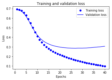
 1 import matplotlib.pyplot as plt
 2
 3 acc = history.history['acc']
 4 val_acc = history.history['val_acc']
 5 loss = history.history['loss']
 6 val_loss = history.history['val_loss']
 7
 8 epochs = range(1,len(acc)+1)
 9
10 plt.plot(epochs,loss,'bo',label='Training loss')#bo为blue dot
11 plt.plot(epochs,val_loss,'b',label='Validation loss')#b 为solid blue line
12 plt.title('Training and validation loss')
13 plt.xlabel('Epochs')
14 plt.ylabel('Loss')
15 plt.legend()
16
17 plt.show()
 1 plt.clf()
 2 acc_values = history_dict['acc']
 3 val_acc_values = history_dict['val_acc']
 4
 5 plt.plot(epochs,acc,'bo',label='Training acc')
 6 plt.plot(epochs,val_acc,'b',label='Validation acc')
 7 plt.title('Training and validation accuracy')
 8 plt.xlabel('Epochs')
 9 plt.ylabel('Accuracy')
10 plt.legend()
11 plt.show()
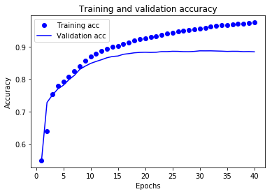
圆点表示训练损失和准确率,实线表示验证损失和准确率。
可以注意到,训练损失随着周期数的增加而降低,训练准确率随着周期数的增加而提高。在使用梯度下降法优化模型时,这属于正常现象 - 该方法应在每次迭代时尽可能降低目标值。
验证损失和准确率的变化情况并非如此,它们似乎在大约 20 个周期后达到峰值。这是一种过拟合现象:模型在训练数据上的表现要优于在从未见过的数据上的表现。在此之后,模型会过度优化和学习特定于训练数据的表示法,而无法泛化到测试数据。
对于这种特殊情况,我们可以在大约 20 个周期后停止训练,防止出现过拟合。
3.召回率、准确率、ROC曲线、AUC、PR曲线基本概念
混淆矩阵:
预测值为正例,记为P(Positive)
预测值为反例,记为N(Negative)
预测值与真实值相同,记为T(True)
预测值与真实值相反,记为F(False)

TP:预测类别是P(正例),真实类别也是P
FP:预测类别是P,真实类别是N(反例)
TN:预测类别是N,真实类别也是N
FN:预测类别是N,真实类别是P
样本中的真实正例类别总数即TP+FN。TPR即True Positive Rate,准确率(查准率):TPR = TP/(TP+FN)
样本中的真实反例类别总数为FP+TN。FPR即False Positive Rate 召回率(查全率):FPR = FP/(TN+FP)
PR曲线:
ROC曲线:
对于一些分类器,分类结果不一定为0,1,可能是概率形式,0.5,0.8...人为定义阈值比如0.4,小于0.4为第0类,大于0.4为第1类,同样这个阈值可以去不同的数值,得到的最后分类情况也不相同。
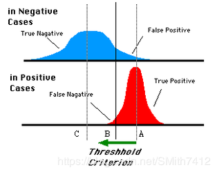
蓝色表示原始为负类分类得到的统计图,红色为正类得到的统计图。那么我们取一条直线,直线左边分为负类,右边分为正,这条直线也就是我们所取的阈值。
阈值不同,可以得到不同的结果,但是由分类器决定的统计图始终是不变的。这时候就需要一个独立于阈值,只与分类器有关的评价指标,来衡量特定分类器的好坏。
还有在类不平衡的情况下,如正样本90个,负样本10个,直接把所有样本分类为正样本,得到识别率为90%。但这显然是没有意义的。
如上就是ROC曲线的动机。
放在具体领域来理解上述两个指标。
如在医学诊断中,判断有病的样本。
那么尽量把有病的揪出来是主要任务,也就是第一个指标TPR,要越高越好。
而把没病的样本误诊为有病的,也就是第二个指标FPR,要越低越好。
不难发现,这两个指标之间是相互制约的。如果某个医生对于有病的症状比较敏感,稍微的小症状都判断为有病,那么他的第一个指标应该会很高,但是第二个指标也就相应地变高。最极端的情况下,他把所有的样本都看做有病,那么第一个指标达到1,第二个指标也为1。
我们以FPR为横轴,TPR为纵轴,得到如下ROC空间。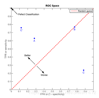
我们可以看出,左上角的点(TPR=1,FPR=0),为完美分类,也就是这个医生医术高明,诊断全对。
点A(TPR>FPR),医生A的判断大体是正确的。中线上的点B(TPR=FPR),也就是医生B全都是蒙的,蒙对一半,蒙错一半;下半平面的点C(TPR<FPR),这个医生说你有病,那么你很可能没有病,医生C的话我们要反着听,为真庸医。
上图中一个阈值,得到一个点。现在我们需要一个独立于阈值的评价指标来衡量这个医生的医术如何,也就是遍历所有的阈值,得到ROC曲线。
还是一开始的那幅图,假设如下就是某个医生的诊断统计图,直线代表阈值。我们遍历所有的阈值,能够在ROC平面上得到如下的ROC曲线。

曲线距离左上角越近,证明分类器效果越好。
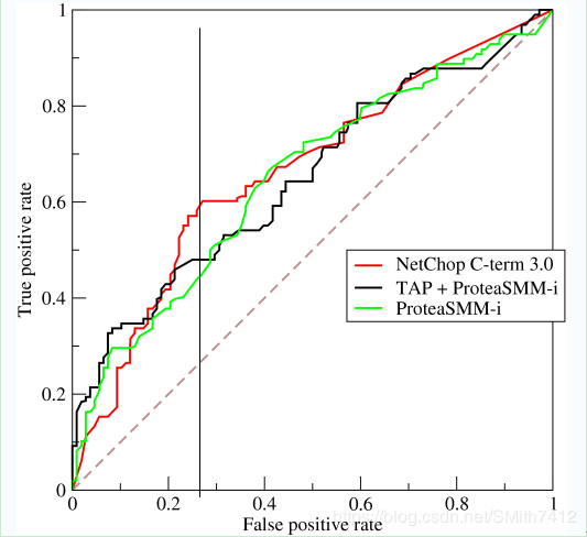
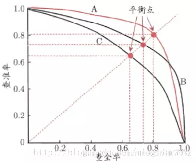
如上,是三条ROC曲线,在0.23处取一条直线。那么,在同样的低FPR=0.23的情况下,红色分类器得到更高的PTR。也就表明,ROC越往上,分类器效果越好。我们用一个标量值AUC来量化他。
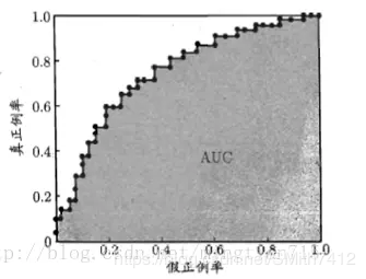
AOC曲线:
AUC值为ROC曲线所覆盖的区域面积,显然,AUC越大,分类器分类效果越好。
AUC = 1,是完美分类器,采用这个预测模型时,不管设定什么阈值都能得出完美预测。绝大多数预测的场合,不存在完美分类器。
0.5 < AUC < 1,优于随机猜测。这个分类器(模型)妥善设定阈值的话,能有预测价值。
AUC = 0.5,跟随机猜测一样(例:丢铜板),模型没有预测价值。
AUC < 0.5,比随机猜测还差;但只要总是反预测而行,就优于随机猜测。
AUC的物理意义
假设分类器的输出是样本属于正类的socre(置信度),则AUC的物理意义为,任取一对(正、负)样本,正样本的score大于负样本的score的概率。
计算AUC:
第一种方法:AUC为ROC曲线下的面积,那我们直接计算面积可得。面积为一个个小的梯形面积之和。计算的精度与阈值的精度有关。
第二种方法:根据AUC的物理意义,我们计算正样本score大于负样本的score的概率。取NM(N为正样本数,M为负样本数)个二元组,比较score,最后得到AUC。时间复杂度为O(NM)。
第三种方法:与第二种方法相似,直接计算正样本score大于负样本的概率。我们首先把所有样本按照score排序,依次用rank表示他们,如最大score的样本,rank=n(n=N+M),其次为n-1。那么对于正样本中rank最大的样本,rank_max,有M-1个其他正样本比他score小,那么就有(rank_max-1)-(M-1)个负样本比他score小。其次为(rank_second-1)-(M-2)。最后我们得到正样本大于负样本的概率为
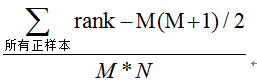
时间复杂度为O(N+M)