欢迎转载,但请务必注明原文出处及作者信息。
深入MNIST
refer: http://wiki.jikexueyuan.com/project/tensorflow-zh/tutorials/mnist_pros.html
@author: huangyongye
@date: 2017-02-24
之前在keras中用同样的网络和同样的数据集来做这个例子的时候。keras占用了 5647M 的显存(训练过程中设了 validation_split = 0.2, 也就是1.2万张图)。
但是我用 tensorflow 自己写的 batch=50 来测试发现呀只有529的占用显存!!!只是在最后做测试的时候因为是对10000多张图片一次性做预测才占用了 8721M 的显存这里的测试集是 1 万张。如果把预测时候的 batch 也设得比较小的话,那么整个网络只需要很小的显存了。
import numpy as np
import tensorflow as tf

# 设置按需使用GPU
config = tf.ConfigProto()
config.gpu_options.allow_growth = True
sess = tf.InteractiveSession(config=config)- 1
- 2
- 3
- 4
- 5
- 6
- 7
1.导入数据,用 tensorflow 导入
# 用tensorflow 导入数据
from tensorflow.examples.tutorials.mnist import input_data
mnist = input_data.read_data_sets('MNIST_data', one_hot=True)- 1
- 2
- 3
Extracting MNIST_data/train-images-idx3-ubyte.gz
Extracting MNIST_data/train-labels-idx1-ubyte.gz
Extracting MNIST_data/t10k-images-idx3-ubyte.gz
Extracting MNIST_data/t10k-labels-idx1-ubyte.gz
- 1
- 2
- 3
- 4
- 5
# 看看咱们样本的数量
print mnist.test.labels.shape
print mnist.train.labels.shape- 1
- 2
- 3
(10000, 10)
(55000, 10)
- 1
- 2
- 3
或者从keras中导入数据
# 注意: keras 中导入数据形式不一样哦,需要根据具体情况调整
from keras.datasets import mnist
(X_train, y_train), (X_test, y_test) = mnist.load_data()
print 'X_train.shape=', X_train.shape
print 'y_train.shape=', y_train.shape

# TensorFlow 类别需要使用 one-hot 类型
from keras.utils import np_utils
y_train = np_utils.to_categorical(y_train)
y_test = np_utils.to_categorical(y_test)
print X_train.shape
print y_train.shape- 1
- 2
- 3
- 4
- 5
- 6
- 7
- 8
- 9
- 10
- 11
- 12
X_train.shape= (60000, 28, 28)
y_train.shape= (60000,)
(60000, 28, 28)
(60000, 10)
- 1
- 2
- 3
- 4
- 5
2. 构建网络
# 权值初始化
def weight_variable(shape):
    # 用正态分布来初始化权值
    initial = tf.truncated_normal(shape, stddev=0.1)
    return tf.Variable(initial)

def bias_variable(shape):
    # 本例中用relu激活函数,所以用一个很小的正偏置较好
    initial = tf.constant(0.1, shape=shape)
    return tf.Variable(initial)

# 定义卷积层
def conv2d(x, W):
    # 默认 strides[0]=strides[3]=1, strides[1]为x方向步长,strides[2]为y方向步长
    return tf.nn.conv2d(x, W, strides=[1,1,1,1], padding='SAME')

# pooling 层
def max_pool_2x2(x):
    return tf.nn.max_pool(x, ksize=[1,2,2,1], strides=[1,2,2,1], padding='SAME')


X_ = tf.placeholder(tf.float32, [None, 784])
y_ = tf.placeholder(tf.float32, [None, 10])

# 把X转为卷积所需要的形式
X = tf.reshape(X_, [-1, 28, 28, 1])
# 第一层卷积:5×5×1卷积核32个 [5,5,1,32],h_conv1.shape=[-1, 28, 28, 32]
W_conv1 = weight_variable([5,5,1,32])
b_conv1 = bias_variable([32])
h_conv1 = tf.nn.relu(conv2d(X, W_conv1) + b_conv1)

# 第一个pooling 层[-1, 28, 28, 32]->[-1, 14, 14, 32]
h_pool1 = max_pool_2x2(h_conv1)

# 第二层卷积:5×5×32卷积核64个 [5,5,32,64],h_conv2.shape=[-1, 14, 14, 64]
W_conv2 = weight_variable([5,5,32,64])
b_conv2 = bias_variable([64])
h_conv2 = tf.nn.relu(conv2d(h_pool1, W_conv2) + b_conv2)

# 第二个pooling 层,[-1, 14, 14, 64]->[-1, 7, 7, 64]
h_pool2 = max_pool_2x2(h_conv2)

# flatten层,[-1, 7, 7, 64]->[-1, 7*7*64],即每个样本得到一个7*7*64维的样本
h_pool2_flat = tf.reshape(h_pool2, [-1, 7*7*64])

# fc1
W_fc1 = weight_variable([7*7*64, 1024])
b_fc1 = bias_variable([1024])
h_fc1 = tf.nn.relu(tf.matmul(h_pool2_flat, W_fc1) + b_fc1)

# dropout: 输出的维度和h_fc1一样,只是随机部分值被值为零
keep_prob = tf.placeholder(tf.float32)
h_fc1_drop = tf.nn.dropout(h_fc1, keep_prob)

# 输出层
W_fc2 = weight_variable([1024, 10])
b_fc2 = bias_variable([10])
y_conv = tf.nn.softmax(tf.matmul(h_fc1_drop, W_fc2) + b_fc2)- 1
- 2
- 3
- 4
- 5
- 6
- 7
- 8
- 9
- 10
- 11
- 12
- 13
- 14
- 15
- 16
- 17
- 18
- 19
- 20
- 21
- 22
- 23
- 24
- 25
- 26
- 27
- 28
- 29
- 30
- 31
- 32
- 33
- 34
- 35
- 36
- 37
- 38
- 39
- 40
- 41
- 42
- 43
- 44
- 45
- 46
- 47
- 48
- 49
- 50
- 51
- 52
- 53
- 54
- 55
- 56
- 57
- 58
3.训练和评估
在测试的时候不使用 mini_batch, 那么测试的时候会占用较多的GPU(4497M),这在 notebook 交互式编程中是不推荐的。
cross_entropy = -tf.reduce_sum(y_*tf.log(y_conv))
train_step = tf.train.AdamOptimizer(1e-4).minimize(cross_entropy)
correct_prediction = tf.equal(tf.argmax(y_conv,1), tf.argmax(y_,1))
accuracy = tf.reduce_mean(tf.cast(correct_prediction, "float"))
sess.run(tf.initialize_all_variables())
for i in range(10000):
    batch = mnist.train.next_batch(50)
    if i%1000 == 0:
        train_accuracy = accuracy.eval(feed_dict={
            X_:batch[0], y_: batch[1], keep_prob: 1.0})
        print "step %d, training accuracy %g"%(i, train_accuracy)
    train_step.run(feed_dict={X_: batch[0], y_: batch[1], keep_prob: 0.5})

print "test accuracy %g"%accuracy.eval(feed_dict={
X_: mnist.test.images, y_: mnist.test.labels, keep_prob: 1.0})- 1
- 2
- 3
- 4
- 5
- 6
- 7
- 8
- 9
- 10
- 11
- 12
- 13
- 14
- 15
WARNING:tensorflow:From <ipython-input-5-94e05db0c125>:5: initialize_all_variables (from tensorflow.python.ops.variables) is deprecated and will be removed after 2017-03-02.
Instructions for updating:
Use `tf.global_variables_initializer` instead.
step 0, training accuracy 0.12
step 1000, training accuracy 0.92
step 2000, training accuracy 0.98
step 3000, training accuracy 0.96
step 4000, training accuracy 1
step 5000, training accuracy 1
step 6000, training accuracy 1
step 7000, training accuracy 1
step 8000, training accuracy 1
step 9000, training accuracy 1
test accuracy 0.9921
- 1
- 2
- 3
- 4
- 5
- 6
- 7
- 8
- 9
- 10
- 11
- 12
- 13
- 14
- 15
下面改成了 test 也用 mini_batch 的形式, 显存只用了 529M,所以还是很成功的。
# 题外话:在做这个例子的过程中遇到过:资源耗尽的错误,为什么?
# -> 因为之前每次做 train_acc  的时候用了全部的 55000 张图,显存爆了.

# 1.损失函数:cross_entropy
cross_entropy = -tf.reduce_sum(y_ * tf.log(y_conv))
# 2.优化函数:AdamOptimizer
train_step = tf.train.AdamOptimizer(1e-4).minimize(cross_entropy)

# 3.预测准确结果统计
# 预测值中最大值(1)即分类结果,是否等于原始标签中的(1)的位置。argmax()取最大值所在的下标
correct_prediction = tf.equal(tf.argmax(y_conv, 1), tf.arg_max(y_, 1))
accuracy = tf.reduce_mean(tf.cast(correct_prediction, tf.float32))


# 如果一次性来做测试的话,可能占用的显存会比较多,所以测试的时候也可以设置较小的batch来看准确率
test_acc_sum = tf.Variable(0.0)
batch_acc = tf.placeholder(tf.float32)
new_test_acc_sum = tf.add(test_acc_sum, batch_acc)
update = tf.assign(test_acc_sum, new_test_acc_sum)

# 定义了变量必须要初始化,或者下面形式
sess.run(tf.global_variables_initializer())
# 或者某个变量单独初始化 如:
# x.initializer.run()

# 训练
for i in range(5000):
    X_batch, y_batch = mnist.train.next_batch(batch_size=50)
    if i % 500 == 0:
        train_accuracy = accuracy.eval(feed_dict={X_: X_batch, y_: y_batch, keep_prob: 1.0})
        print "step %d, training acc %g" % (i, train_accuracy)
    train_step.run(feed_dict={X_: X_batch, y_: y_batch, keep_prob: 0.5})

# 全部训练完了再做测试,batch_size=100
for i in range(100):
    X_batch, y_batch = mnist.test.next_batch(batch_size=100)
    test_acc = accuracy.eval(feed_dict={X_: X_batch, y_: y_batch, keep_prob: 1.0})
    update.eval(feed_dict={batch_acc: test_acc})
    if (i+1) % 20 == 0:
        print "testing step %d, test_acc_sum %g" % (i+1, test_acc_sum.eval())
print " test_accuracy %g" % (test_acc_sum.eval() / 100.0)- 1
- 2
- 3
- 4
- 5
- 6
- 7
- 8
- 9
- 10
- 11
- 12
- 13
- 14
- 15
- 16
- 17
- 18
- 19
- 20
- 21
- 22
- 23
- 24
- 25
- 26
- 27
- 28
- 29
- 30
- 31
- 32
- 33
- 34
- 35
- 36
- 37
- 38
- 39
- 40
- 41
step 0, training acc 0.16
step 500, training acc 0.9
step 1000, training acc 0.98
step 1500, training acc 0.96
step 2000, training acc 1
step 2500, training acc 0.98
step 3000, training acc 1
step 3500, training acc 0.96
step 4000, training acc 1
step 4500, training acc 1
testing step 20, test_acc_sum 19.65
testing step 40, test_acc_sum 39.21
testing step 60, test_acc_sum 58.86
testing step 80, test_acc_sum 78.71
testing step 100, test_acc_sum 98.54
 test_accuracy 0.9854
- 1
- 2
- 3
- 4
- 5
- 6
- 7
- 8
- 9
- 10
- 11
- 12
- 13
- 14
- 15
- 16
- 17
4. 查看网络中间结果
在学习 CNN 的过程中,老是看到他们用图片的形式展示了中间层卷积的输出。好吧,这下我必须得自己实现以下看看呀!!!
关于 python 图片操作主要有 matplotlib 和 PIL 两个库(refer to: http://www.cnblogs.com/yinxiangnan-charles/p/5928689.html)。
我们使用 matplotlib 来完成这个任务。
4.1 图像操作基础
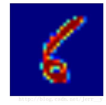
# 我们先来看看数据是什么样的
img1 = mnist.train.images[1]
label1 = mnist.train.labels[1]
print label1  # 所以这个是数字 6 的图片
print 'img_data shape =', img1.shape  # 我们需要把它转为 28 * 28 的矩阵
img1.shape = [28, 28]- 1
- 2
- 3
- 4
- 5
- 6
[ 0.  0.  0.  0.  0.  0.  1.  0.  0.  0.]
img_data shape = (784,)
- 1
- 2
- 3
import matplotlib.pyplot as plt
# import matplotlib.image as mpimg  # 用于读取图片,这里用不上

print img1.shape- 1
- 2
- 3
- 4
(28, 28)
- 1
- 2
plt.imshow(img1)
plt.axis('off') # 不显示坐标轴
plt.show() - 1
- 2
- 3
plt.imshow?- 1
好吧,是显示了图片,但是结果是热度图像。我们想显示的是灰度图像。
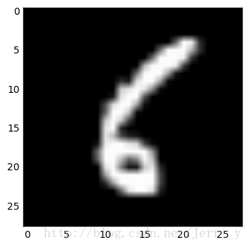
# 我们可以通过设置 cmap 参数来显示灰度图
plt.imshow(img1, cmap='gray') # 'hot' 是热度图
plt.show()- 1
- 2
- 3
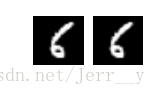
我们想看 Conv1 层的32个卷积滤波后的结果,显示在同一张图上。 python 中也有 plt.subplot(121) 这样的方法来帮我们解决这个问题。如下:先看两个试试
plt.subplot?- 1
img1.shape- 1
(1, 784)
- 1
- 2
plt.subplot(4,8,1)
plt.imshow(img1, cmap='gray')
plt.axis('off')
plt.subplot(4,8,2)
plt.imshow(img1, cmap='gray')
plt.axis('off')
plt.show()- 1
- 2
- 3
- 4
- 5
- 6
- 7
4.2 显示网络中间结果
好了,有了前面的图像操作基础,我们就该试试吧!!!
# 首先应该把 img1 转为正确的shape (None, 784)
X_img = img1.reshape([-1, 784])
y_img = mnist.train.labels[1].reshape([-1, 10])
# 我们要看 Conv1 的结果,即 h_conv1
result = h_conv1.eval(feed_dict={X_: X_img, y_: y_img, keep_prob: 1.0})
print result.shape
print type(result)- 1
- 2
- 3
- 4
- 5
- 6
- 7
(1, 28, 28, 32)
<type 'numpy.ndarray'>
- 1
- 2
- 3
好的,我们成功的计算得到了 h_conv1,那么赶紧 imshow() 看看吧!!!
for _ in xrange(32):
    show_img = result[:,:,:,_]
    show_img.shape = [28, 28]
    plt.subplot(4, 8, _ + 1)
    plt.imshow(show_img, cmap='gray')
    plt.axis('off')
plt.show()- 1
- 2
- 3
- 4
- 5
- 6
- 7
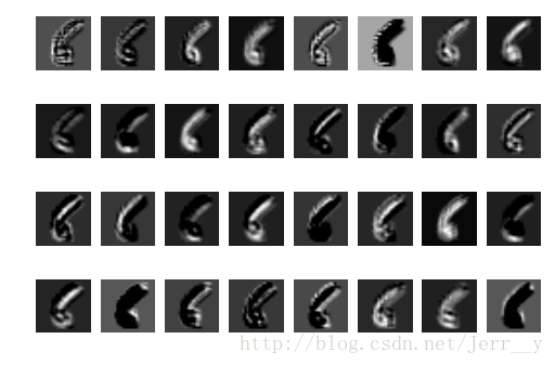
哈哈,成功啦!从上面的结果中,我们可以看到不同的滤波器(卷积核)学习到了不同的特征。比如第一行中,第一个滤波器学习到了边缘信息,第5个卷积核,则学习到了骨干的信息。感觉好有趣,不由自主的想对另一个数字看看。
# 输出前10个看看,我选择数字 9 来试试
print mnist.train.labels[:10]- 1
- 2
[[ 0.  1.  0.  0.  0.  0.  0.  0.  0.  0.]
 [ 0.  0.  0.  0.  0.  0.  1.  0.  0.  0.]
 [ 0.  0.  0.  0.  0.  0.  0.  0.  0.  1.]
 [ 0.  0.  0.  0.  0.  0.  0.  1.  0.  0.]
 [ 0.  0.  0.  0.  0.  1.  0.  0.  0.  0.]
 [ 0.  1.  0.  0.  0.  0.  0.  0.  0.  0.]
 [ 0.  0.  1.  0.  0.  0.  0.  0.  0.  0.]
 [ 0.  0.  0.  1.  0.  0.  0.  0.  0.  0.]
 [ 0.  0.  0.  0.  0.  0.  0.  0.  0.  1.]
 [ 0.  0.  0.  0.  0.  0.  0.  0.  0.  1.]]
- 1
- 2
- 3
- 4
- 5
- 6
- 7
- 8
- 9
- 10
- 11
# 首先应该把 img1 转为正确的shape (None, 784)
X_img = mnist.train.images[2].reshape([-1, 784])
y_img = mnist.train.labels[1].reshape([-1, 10]) # 这个标签只要维度一致就行了
result = h_conv1.eval(feed_dict={X_: X_img, y_: y_img, keep_prob: 1.0})

for _ in xrange(32):
    show_img = result[:,:,:,_]
    show_img.shape = [28, 28]
    plt.subplot(4, 8, _ + 1)
    plt.imshow(show_img, cmap='gray')
    plt.axis('off')
plt.show()- 1
- 2
- 3
- 4
- 5
- 6
- 7
- 8
- 9
- 10
- 11
- 12

第一个核还是主要学习到了边缘特征,第五个核还是学到了骨干特征(当然在某种程度上)。好吧,本次就到这啦!