Machine Learning(week 7~11)

Support Vector Machines

Large Margin Classification

1. Optimization Objective

Support vector machine (SVM): a supervised learning algorithm, sometimes gives cleaner, more powerful ways of learning complex non-linear algorithm than logistic regression and neural network.

Modify logistic regression to get SVM

In logistic regression: (as we have known)

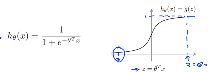
If y=1, we want h_θ(x)≈1, i.e. θ^Tx>>0;

If y=0, we want h_θ(x)≈0, i.e. θ^Tx<<0.

A single example’s contribution to the overall cost:

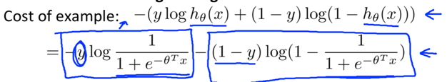
 when y=1 or y=0, only one of the terms matters: (z=θ^Tx)

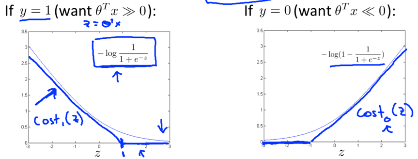
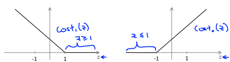
Build a new function: a straight line and a flat line, joining at x=1 (when y=1, the function is called cost₁(z).) or x=-1 (when y=0, the function is called cost₀(z).).

Replace these terms with cost₁(z) and cost₀(z) in the logistic regression cost function:

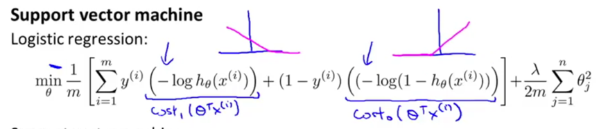
A minimization problem for SVM:

 

Use the notational convention for SVM instead:

1. get rid of 1/m; 2. Use a different way to control the trade off: A+λB –> CA+B. 

(regularization parameter C plays a similar role as 1/λ, should give the same optimal value for θ.)

Finally, the overall optimization objective function (i.e. cost function) for SVM: (minimize it to get the parameters learned by SVM)

h_θ(x) for SVM doesn’t output the probability, it makes prediction (y=1 if θ^Tx>=0, otherwise y=0) directly.

2. Large Margin Intuition

 To minimize the cost function for SVM: (when C is very large, I guess.)

If y=1, we want θ^Tx>=1 (not just >=0);

If y=0, we want θ^Tx<=-1 (not just <0).

-- SVM doesn’t just barely get the example right, an extra safety margin factor is built into SVM.

Decision boundary: 

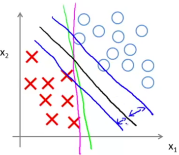
 The decision boundary given by SVM (in black) has a larger minimum distance from training examples than the magenta or green one.

The distance between blue and black is called the margin of the SVM, it gives SVM a certain robustness. SVM is also called large margin classifier, it tries to separate the positive and negative examples with as big margin as possible (only when C is very large).

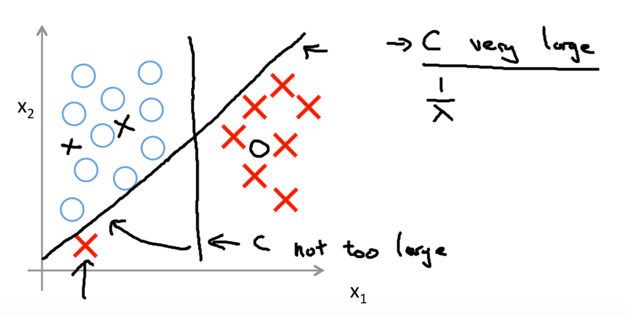
If C very is large, the learning algorithm will sensitive to outliers;

If C is reasonably small, the decision boundary will do a better job ignoring the few outliers.

(The same applies to nonlinear problem.)

3. Mathematics Behind Large Margin Classification

Vector inner product

Given two vectors u and v, u^Tv is called the inner product between u and v.

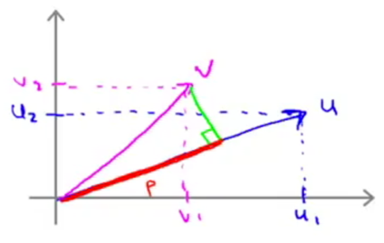
p is the length of the orthogonal projection of v onto u. p is signed, if the angle between u and v is greater than 90°, p will be negative.

Given a vector u, the norm of u is ||u||=, is the length of u.

u^Tv = p·||u|| = v^Tu = u₁v₁+u₂v₂

(||u||, p∈R.)

How SVM leads to large margin classifier:

To simplify, set θ₀=0, the number of features n=2.

The optimization objective of SVM (when C is very large):

 (because θ₀=0),

so SVM is trying to minimize the square length of θ

Apply inner product understanding to θ^Tx⁽ⁱ⁾:

 

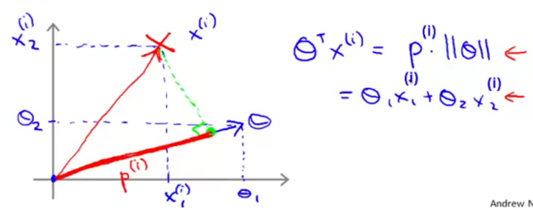
-> The constraints 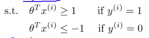 can be replaced with p⁽ⁱ⁾·||θ||: (p⁽ⁱ⁾is the projection of x⁽ⁱ⁾onto θ.)

1) If choosing a decision boundary with small margins (which in fact SVM would not choose):

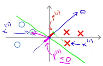
θ is always at 90°to the decision boundary.

For some example x⁽ⁱ⁾that is close to the decision boundary, p⁽ⁱ⁾ is going to be pretty small (the absolute value). Then to satisfy the constraints, we need ||θ|| to be large, which is contradictory to the optimization objective of SVM.

2) If choosing a decision boundary with large margins:

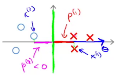
p⁽ⁱ⁾ is going to be much bigger, then ||θ|| can be smaller, which is SVM is going to choose.

Because the only way to make p(i) to be large is let the decision boundary have large margins.

θ₀=0 means the decision boundary must pass (0,0). The proof works the same for θ₀≠0.

 

Kernels 

Problem-> To learn a non-linear decision boundary, is there a different/better choice of those high-order polynomials features (f1, f2, f3, ….)?

e.g. predict y=1 if θ₀+θ₁f₁+θ₂f₂+θ₃f₃+…>=0, where f₁=x₁, f₂=x₂, f₃=x₁x₂, f₄=x₁², ….

Solution->

Manually pick landmarks, compute f_i:

(||x-l⁽ⁱ⁾|| is the Euclidean distance between point x and l⁽ⁱ⁾, ingoring x₀).

Kernel: usually written as k(x, l⁽ⁱ⁾), are similarity() functions defined to measure the similarity between example x and the ith landmark, can have many different forms. The similarity() used here is a Gaussian kernel function.

f_imeasures how close x is to the ith landmark.

 

e.g. to define features f₁, f₂, f₃:

Manually pick 3 points (landmarks): l⁽¹⁾, l⁽²⁾, l⁽³⁾on x₁*x₂space;

Given x and the 3 landmarks, we can compute new features f1, f2, f3

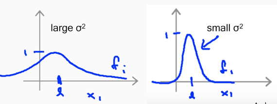
The plot of f_i:

e.g. given x₁, x₂and l⁽¹⁾, plot f₁:

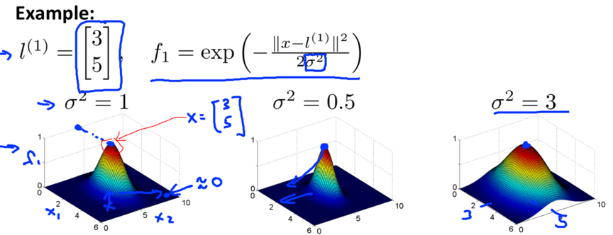
contour plot:

sigma square is the parameter of the Gaussian kernel. When sigma square is small, the width of the bump is narrower, the contour shrinks, f_i falls to 0 more rapidly.

SVM with kernel can be a powerful way to learn complex non-linear function.

How to choose landmarks?

Put landmarks at exactly the same location as the training examples.

i.e. Given (x⁽¹⁾,y⁽¹⁾), (x⁽²⁾, y⁽²⁾), …, (x^(m), y^(m)), choose l⁽¹⁾=x⁽¹⁾, l⁽²⁾=x⁽²⁾, …, l^(m)=x^(m).

-> Given an example x (in training set/cross-validation set or test set), we can compute a feature vectors f=, where f_i=similarity(x,l⁽ⁱ⁾)=(x,x⁽ⁱ⁾), x(i) is the ith example in the training set. (can also add a f₀=1)

-> For training example (x⁽ⁱ⁾,y⁽ⁱ⁾), there will be f_i⁽ⁱ⁾=similarity(x⁽ⁱ⁾,x⁽ⁱ⁾)=1.

Instead of using x(i)∈Rⁿ⁺¹, now we can represent the example using feature vectors 

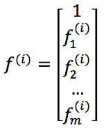, (f0(i)=1 as convention.)

How to make predictions (using SVM with kernels)

Given θ∈R^m+1 (that has been learned) and x,

-> compute f∈R^m+1,

-> predict y=1 if θ^Tf≥0

How to get θ (using SVM with kernels)

-> Solve this minimization problem:

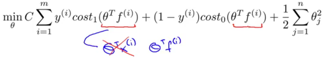
 compared to the cost function for SVM, it replaces θ^Tx⁽ⁱ⁾ with θ^Tf⁽ⁱ⁾.

one last detail:

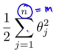-the n in this term is actually equal to m, (we do not regularize θ₀).

In the actual implementation of SVM, the = θ^Tθ (again, we ignore θ₀, so θ= here) in this term is replaced by θ^TMθ, where M is some matrix depends on the kernel being used.  

It improves SVM’s computational efficiency (because it allows SVM to scale to much bigger training sets).

If you want, you can apply kernel to logistic regression, but it will run very slowly (because the idea of kernels is particularly designed for SVM, it goes well with SVM but don’t generalize well to other algorithms).

How to choose parameters for SVM 

1) C (=1/λ)

Large C -> low bias, high variance, is prone to overfitting;

Small C -> high bias, low variance is prone to underfitting.

2) σ² (in Gaussian kernel)

Large σ²-> features f_ivary smoothly, the hypothesis has high bias, low variance.

Small σ²-> features f_ivary abruptly, the hypothesis has low bias, high variance.

 

SVM in practice

It is recommended to use SVM software package (e.g. liblinear, libsvm) to solve SVM optimization problem (i.e. solve for θ) rather than implement it yourself.

Need to specify: 1) parameter C; 2) kernel.

Two common choice for kernel:

1. Linear kernel: no kernel, use SVM that just predict y=1 if θ^Tx≥0 so it will gives a standard linear classifier. Linear kernel is suitable for situations when n (the number of features) is large and m (the number of training examples) is small.

2. Gaussian kernel, where l⁽ⁱ⁾=x⁽ⁱ⁾, need to choose σ². Is suitable for situations when n is small and m is large.

 

If there are features of very different sales, feature scaling should be performed before using Gaussian kernel.

Reason: the || x-l ||²term in the Gaussian kernel function = (x₁-l₁)²+(x₂-l₂)²+…+(x_n-l_n)², if one feature is in a large range (e.g. x₁, 1000 feet²) but another feature is in a small range (e.g. x₂, 5 bedrooms), then this distance term will be dominated by one feature and another feature will be largely ignored.

(I think the subscript i here does not mean the ith landmark we usually denote, it means the ith feature of the one landmark l.)

Feature scaling ensures SVM gives comparable amount of attention to all features.

 

Note: Not all similarity function make valid kernels.

All kernels need to satisfy “Mercer’s Theorem”to make sure SVM packages’ optimization run correctly and do not diverge.

Some other kernels: 

- Polynomial kernel: k(x, l)=(x^Tl+some constant)^{some degree},when x and l are similar, the inner product x^Tl tends to be large. E.g. k(x,l)=(x^Tl)², (x^Tl)³, (x^Tl+1)³or (x^Tl+5)⁴, etc. Usually is used only when X and l are all strictly non-negative (to ensures the inner product is never negative).

- String kernel: used when input data is text string or other strings.

- chi-string kernel, histogram intersection kernel, etc.

 

Multi-class classification in SVM

1. Many SVM package already have built-in multi-class classification functionality.

2. Otherwise, use one-vs-all method:

- Train K SVMs, each one to distinguish its class (y=i) from the rest

- gain K parameter vectorsθ⁽¹⁾, θ⁽²⁾, …, θ^(K), each θ⁽ⁱ⁾have y=I as the positive class and all the others as negative class.

- pick a class i with the largest (θ⁽ⁱ⁾)^Tx.

(here it means just predict y=i with (θ⁽ⁱ⁾)^Tx. However, personally I think we should take SVM with kernels into considerations. For SVM with kernels, we predict y=1 if θ^Tf≥0, so I think we should pick a class i with the largest (θ⁽ⁱ⁾)^Tf if the ith SVM we trained use a kernel.)

 

Logistic regression vs. SVMs

n: number of features;

m: number of training examples.

n is large (relative to m). e.g. n=10000, m∈[10, 1000]

-> Use logistic regression, or SVM without a kernel (i.e. linear kernel). Because you don’t have enough data to fit a complex nonlinear function, a linear function is just fine.

n is small, m is intermediate. e.g. n∈[1, 1000], m∈[10, 10000]

-> Use SVM with Gaussian kernel.

n is small, m is large. e.g. n∈[1, 1000], m>=50000

-> Create/add more features, then use logistic regression or SVM without a kernel. (Because SVM with Gaussian kernel will be slow with a massive training set.)

logistic regression and SVM without a kernel are pretty similar algorithms, they usually have similar performance.

A well-designed neural network can work well for most of the settings, but may be slower to train. On the contrary, with a good SVM package,SVM can run much faster.

SVM has a convex optimization problem, so you don’t need to worry about local optima. (local optima isn’t a big problem for neural network either, but SVM remains a better method for these 3 regimes because it’s faster.)

 

Unsupervised Learning

Clustering

1. unsupervised Learning

Unsupervised learning: Given unlabelled training set (i.e. no labels y given), ask the algorithm to find some structure in the data.

Clustering algorithm: a type of unsupervised learning algorithm that find clusters type structure in the data.

2. K-Means Algorithm– a popular clustering algorithm

Input:

1) K = number of clusters

2) Training set {x⁽¹⁾, x⁽²⁾, …, x^(m)}. Notice that the x0=1 convention is dropped thus x⁽ⁱ⁾∈Rⁿ.

Algorithm cluster assignment step + move centroid step

Randomly initialize K cluster centroids μ1, μ2, …, μK∈Rn.
Repeat {
  [cluster assignment step]
  for i = 1 : m
c(i) := index (from 1 to K) of cluster centroid closest to x(i)
// i.e. c(i)=the value of k that minimize ||x(i)-μk||², the lowercase k denote a number in [1, K].
  [move centroid step]
  for k = 1 : K
    μK := average (mean) of points assigned to cluster k
}

Problem: What if for a specific cluster with 0 point assigned to it?

Solution: Generally, just eliminate that cluster centroid -> end up with K-1 clusters; If you really need K clusters, just randomly reinitialize that cluster centroid.

3. Optimization Objective

c⁽ⁱ⁾: index of cluster (1, 2, …, K) to which x⁽ⁱ⁾is currently assigned.

μ_K: the cluster centroid k, ∈R.

μ_c⁽ⁱ⁾: the cluster centroid of cluster to which example x⁽ⁱ⁾ has been assigned.

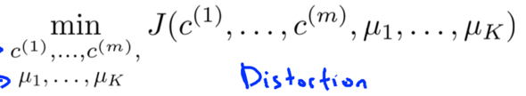
Optimization Objective for K-means algorithm: a.k.a. the Distortion of the K-means algorithm.

tries to find c and mu that minimize the cost function J

In the K-means algorithm,

What the [cluster assignment step] does is to minimize J with respect to c⁽¹⁾,  …, c^(m); (hold μ fixed to pick c that minimize J)

What the [move centroid step] does is to minimize J with respect to μ₁, …, μ_K.

4. Random Initialization

Recommended approach:

Have K<m, m is the number of training examples.

Randomly pick K training examples, then set μ₁, …, μ_K equals to these K examples.

Problem: Depending on the random initialization, K-means algorithm can end up at different solutions. -> local optima.

Solution: Try multiple random initializations, trying to make sure we get a good solution.

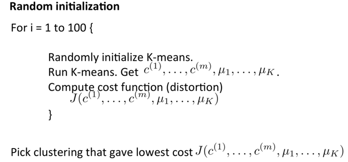
(Usually run K-means for 50~1000 times)

If running K-means with a small number of clusters (e.g. K∈[2, 10]), then multiple random initialization sometimes makes sure you find a better local optima. But if K is very large, multiple random initialization is less likely to make a difference.

5. Choosing the Number of Clusters

1. Elbow method - is worth a shot, but we won’t have a very high expectation of it working on any particular problem.

Run K-means with different K, plot how distortion varies along with K. Find the “elbow”of the curve, where the distortion goes down rapidly.

 

Elbow method isn’t used very often, because there usually isn’t a clear elbow: 

2. Ask: which K serves the latter purpose best? (a better approach)

Sometimes people run K-means to get clusters for some later/downstream purpose. (E.g. market segmentation in T-shirt sizing.) If that later/downstream purpose gives an evaluation metric, we can determine the number of clusters based on how well different K serve that later downstream purpose. (E.g. think from the perspective of the T-shirt business: Whether I want more T-shirt sizes thus they fit customers better or I want fewer sizes so I can sell them more cheaply?)

For the most part, K is still chosen by hand.

  

Dimensionality Reduction

Motivation

1. Motivation I: Data Compression

Dimensionality Reduction: a type of unsupervised learning problems. When having many features, some of them might be highly redundant or correlative, so we expect to reduce the dimension of the data.

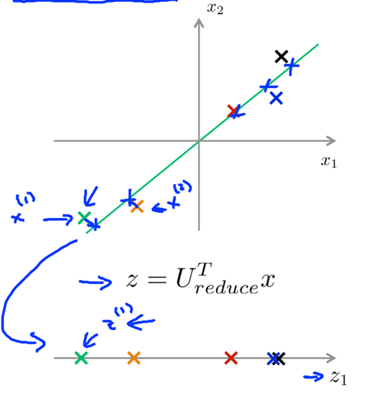
e.g. 2D->1D

-> find a line on which most of the data seem to lie, project all data onto that line 

-> new features z₁specifies the location of each of those points on that line

e.g. 3D->2D

-> originally, most data are roughly lies on some 2D plane

-> project all data onto a 2D plane

-> new features z₁and z₂specify the location of a point within the plane

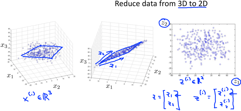
Typical reductions are like 1000D->100D, just that 3D->2D or 2D->1D is easier to plot as examples.

2. Motivation II: Visualization

e.g.

-> originally: 50 features

-> dimension reduction: 50D->2D or 3D. (it’s often up to us to figure out roughly what these new features mean.)

-> can plot the data thus understand it better.

 

Principal Component Analysis

1. Principal Component Analysis Problem Formulation– what we would like PCA to do

Principal Component Analysis (PCA): the most popular algorithm used in dimension reduction. 

The goal of PCA -> (When Reducing data from n-dimension to k-dimension) Find k vectors u⁽¹⁾, u⁽²⁾, …, u^(k)onto which to project the data so as to minimize the projection error.

“Project the data” means to project the data onto the linear subspace spanned by that k vectors.

e.g. 

For 2D->1D, PCA aims to find a direction (a vector u⁽¹⁾∈R²) onto which to project the data so as to minimize the projection error.

For 3D->2D, PCA aims to find 2 vectors to define surface onto which to project the data, …. 

p.s. whether PCA gives u^(k)or –u^(k) doesn’t matter.

e.g.

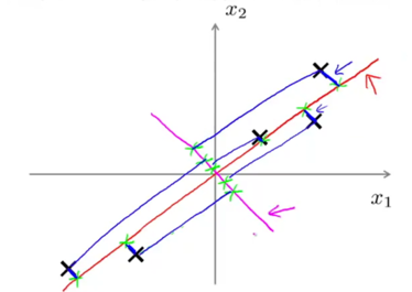
-> originally: x∈R2, we want to reduce x to 1D.

-> PCA will choose the red line rather than the magenta line.

Projection error: the distance between the original data and its projected version.

What PCA does is trying to find a lower dimensional surface (e.g. the line in the example), onto which to project data so that the sum of (projection error)²is minimized.

PCA is not linear regression, they are totally different algorithms.

Linear regression-> there is distinguished variable y we are trying to predict.

PCA -> there is no distinguished variable y, all features x₁, x₂, …, x_nare treated equally.

e.g.

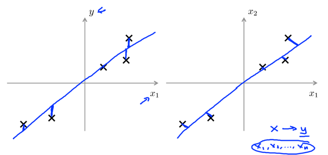
linear regression tries to minimize the square magnitude of the vertical distance between the points and their predicted values;

PCA tries to minimize the square magnitude of the shortest orthogonal distance between the points and the line.

2. Principal Component Analysis Algorithm

Given training set: x(¹⁾, x⁽²⁾, …, x^(m);

Preprocessing: Perform feature scaling & mean normalization on x

1) compute the mean of each feature:  ;

2) Replace each feature x_j⁽ⁱ⁾with x_j-u_j. (thus each feature has mean=0)

3) If different features have different scales, scale features to have comparable range of values: 

 , s_jis some measure of the range of values of x_j, e.g. max(x_j)-min(x_j), standard deviation of x_j, etc.

What PCA Algorithm does:

e.g. 

2D->1D: x(i)∈R²->find vector u⁽¹⁾, get z⁽ⁱ⁾∈R

3D->2D: x(i)∈R³->find vectors u⁽¹⁾and u⁽²⁾, get z⁽ⁱ⁾∈R²

PCA needs to compute vectors u (u⁽¹⁾, u⁽²⁾…) and z (z⁽¹⁾, z⁽²⁾, …).

PCA Algorithm - To reduce data from n-dimensions to k-dimensions:

1) Compute the covariance matrix: 

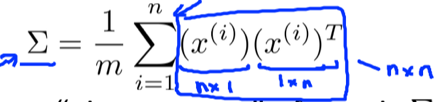
If X is given like: , the computation of covariance matrix in octave can be implemented as:

Sigma = (1/m)* X’ * X;

2) computing the eigenvectors of matrix sigma:

in octave:

 [U, S, V] = svd(Sigma);

svd: singular value decomposition

octave function eig() can also compute the same eigenvectors of covariance matrix sigma, just svd is a little more numerically stable.

If implementing this in languages other than Octave or Matlab, find a numerical linear algebra library that computes svd.

3) Get u (an n*n matrix) whose columns are exactly vectors u⁽¹⁾, u⁽²⁾, …, u⁽ⁿ⁾. Construct an n*k matrix U_reduce=[u(1), u(2), …, u(k)].

 

Take the first k vectors u⁽¹⁾, u⁽²⁾, …, u^(k)as the k directions onto which we want to project the data.

In octave:

Ureduce = U(:, 1:k);

4) Compute the z=U_reduced^Tx , z’s dimension is k*n * n*1=k*1. The x here can be examples in training set, cross validation set or test set.

In ocatave:

Z = Ureduce’ * x;

Similar with k-means, this is not done with x₀=1.

Applying PCA

1. Reconstruction from Compressed Representation

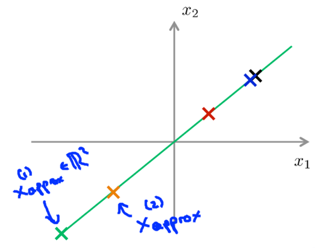
-- to reconstruct an approximation of the original high-dimensional data x from the compressed representation z.

x_approx=U_reduce*z, x_approx’s dimension is n*k * k*1=n*1.

e.g. 

 1D->2D: z∈R->x∈R²

->

2. Choosing the Number of Principal Components

PCA: n-dimension->k-dimensional. k is called the number of principal components.

How to choose parameter k for PCA

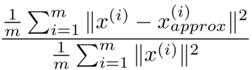
Average squared projection error: , which PCA tries to minimize.

Total variation in the data: .

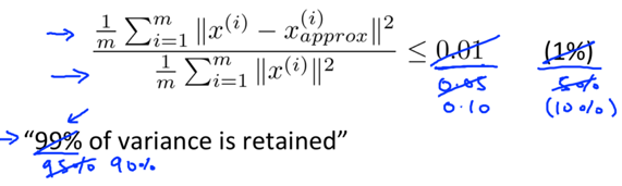
Typically, choose k to be the smallest value so that:

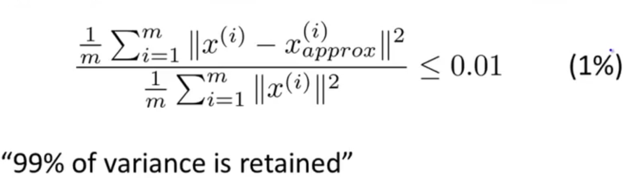-> this indicates how well your reduced dimensional representation is approximating your original data.

other common values can be in [0.05, 0.10], etc.

Most high dimensional data sets tend to have highly correlated features, so PCA can often retain high fraction of variance (e.g. 99%) even while compressing the data by a very large factor.

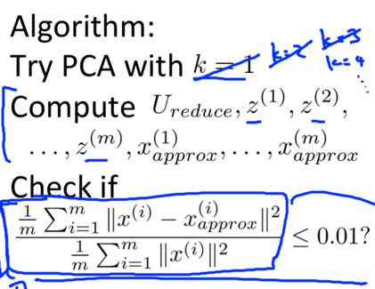
algorithm of choosing k

An inefficient algorithm:

1) start off with k=1;

2) run PCA: compute U_reduce, z⁽¹⁾, z⁽²⁾, …, z^(m), x⁽¹⁾_approx, …, x^(m)_aprrox;

3) check if 99% of variance is retained, 

  if yes -> use k=1 and end;

  if no -> k++, try again until 99% of variance is retained.

Make the computation easier: - need to call svd() only once.

1) Call svd: [U, S, V] = svd(Sigma) to get an n*n diagonal matrix S:

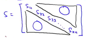
2) Pick the smallest value of k which satisfies:

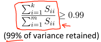
explanation-> For a given k,

 is equal to: .

3. Advice for Applying PCA

Use PCA to speed up supervised learning

PCA reduce the dimensions of the data -> speed up the algorithm

e.g. Input: (x⁽¹⁾, y⁽¹⁾), (x⁽²⁾, y⁽²⁾), …, (x^(m), y^(m)), where x⁽ⁱ⁾∈R¹⁰⁰⁰⁰.

1) Extract input -> get unlabelled dataset x⁽¹⁾, x⁽²⁾, …, x^(m)∈R10000.

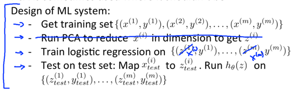
2) Apply PCA -> get reduced dimension representation z⁽¹⁾, z⁽²⁾, …, z^(m)∈R1000.

3) Get new training set (z⁽¹⁾, y⁽¹⁾), (z⁽²⁾, y⁽²⁾), …, (z^(m), y^(m)), feed it to a learning algorithm to learn hypothesis h_θ(z).

4) For a new example, map through the same mapping found by PCA to get its corresponding z, make prediction by computing h_θ(z).

Note: Mapping: x⁽ⁱ⁾->z⁽ⁱ⁾should be defined by running PCA only on the training set, not cross-validation set or test set. This mapping can then be applied to examples in the cross-validation set or test set.

Application of Dimensionality Reduction

1. Data Compression: Reduce memory/disk needed to store data; Speeds up the learning algorithm;

2. Visualization. -> we usually choose k=2 or k=3 to plot the data.

Bad use of PCA: try to use it to prevent overfitting

This might work OK, but is not a good way to address overfitting, regularization should be used instead.

Reason -> PCA does not use the labels y, it might throw away some valuable information, while the cost function with regularization won’t.

Try with the original data x(i) before implementing PCA – Don’t incorporate PCA into the plan in the beginning.

Ditch the PCA step firstly, train the algorithm on the original data. Only if that doesn’t work (e.g. algorithm runs too slowly, memory/disk requirement is too large) then implement PCA and use the compressed z⁽ⁱ⁾.

Anomaly Detection

 Density Estimation

 1. Problem Motivation

 Anomaly detection problem: Given dataset {x⁽¹⁾, x⁽²⁾, …, x^(m)}, usually assume that these m examples are normal, tell if some new example x_test is anomalous.

 Approach->Given the unlabelled training set, build a model p(x).If p(x_test)<ε, x_test is flagged as anomaly.

 2. Gaussian Distribution

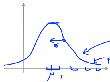
 Gaussian Distribution: a.k.a. Normal Distribution. x～N(μ, σ²) represents x∈R is a distributed Gaussian with mean μ, variance σ².(σ: standard deviation)

σ usually indicates the half-width of the shape.

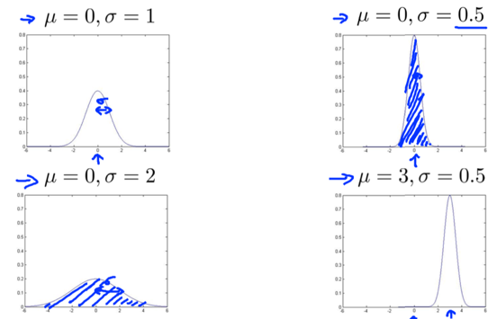
 Plot: the probability of x taking on different values (which is parameterized by μ and σ².) 

 

Formula: 

e.g.

 Parameter estimation problem: Given dataset { x⁽¹⁾, x⁽²⁾, …, x^(m)}, x⁽ⁱ⁾∈R, suspect that x⁽ⁱ⁾～N(μ, σ²), to estimate the unknown values of μ and σ².

-> Formula (the maximum likelihood estimate of μ and σ²):

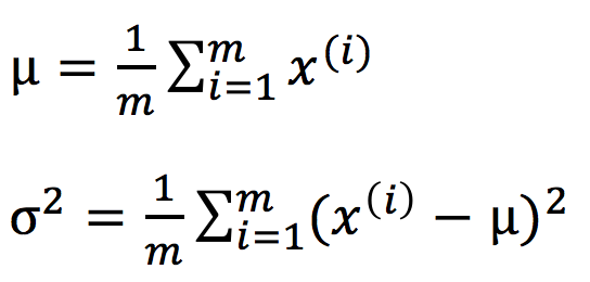
maximum likelihood estimate might use 1/(m-1) instead of 1/m, but in machine learning people tend to use 1/m. In practice they makes little difference assuming m is very large.

3. Algorithm

Density estimation

Input: training set {x⁽¹⁾, x⁽²⁾, …, x^(m)}, x⁽ⁱ⁾∈Rⁿ.

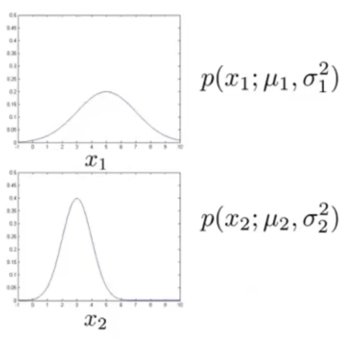
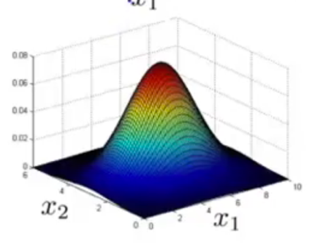
Approach: x_i is a feature of x, assumes x_i～N(μ_i, σ_i²),

model 

This problem of estimating P(x) is called the problem of density estimation.

Anomaly detection algorithm

1) Choose features x_i that you think might be indicative of anomalous examples. I.e. x_i might take on unusually large/small values for anomaly examples. (I guess this step is just pick out features x₁, x₂, …, x_n for x)

2) Fit parameters μ₁, …, μ_n, σ₁², …, σ_n² to the given dataset {x⁽¹⁾, x⁽²⁾, …, x^(m)}:

(compute through j=1:n) -> Formula:

 

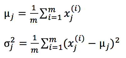
A Vectorized version: (σ² can be computed vectorizely as well.)

3) Given new example x, compute , flag x as anomaly if p(x)<ε. 

 e.g. 

 -> 

All values of x that have a lower height than ε are flagged as anomaly.

 

Building an Anomaly Detection System

1. Developing and Evaluating an Anomaly Detection System

Evaluate the performance of an anomaly detection system

-> Assume we have some labelled data of anomalous (y=1) and non-anomalous (y=0) examples.

(Unlabelled) training set: x⁽¹⁾, x⁽²⁾, …, x^(m), usually assume the majority is non-anomalous.

-> Then define cross validation set and test set to evaluate the algorithm

Cross validation set: (x_cv⁽¹⁾, y_cv⁽¹⁾), …, (x_cv^(m), y_cv^(m))

Test set: (x_test⁽¹⁾, y_test⁽¹⁾), …, (x_test^(m), y_test^(m))

e.g.

10000 normal examples and 20 anomalous examples.

-> Split them into different set:

Training set: 6000 normal examples; (unlabelled, but actually we know they are all y=0)

Cross validation set: 2000 y=0 examples, 10 y=1 examples;

Test set: 2000 y=0 examples, 10 y=1 examples.

-> Use the training set to fit p(x) = p(x₁; μ₁, σ₁²)… p(x_n; μ_n, σ_n²), get μ₁, …, μ_n, σ₁², …, σ_n².

Alternatively, sometimes people use same y=0 or y=1 data in cross validation set and test set, but this is less recommended. E.g. 6000 y=0 examples for training set, same 4000 y=0 examples and different each 10 y=1 examples for both CV and Test set. 

-> Fit model p(x) on training set.

-> On a cross validation set or test set example x, predict:

     y=1 (anomaly) if p(x)<ε;

     y=0 (normal) if p(x)≥ε;

-> Possible evaluation metrics: (because y=0 is much more common, the data will be skewed.)

     True positive, false positive, false negative, true negative;

     Precision, Recall;

     F₁-score.

Cross validation set: used to make decisions (what features to include, choose parameter ε): e.g. try different values of ε, pick the one that maximize F₁-score.

Test set: used to evaluate the final model.

2. Anomaly Detection vs. Supervised Learning -Under which condition should we choose anomaly detection or supervised learning

Anomaly Detection:

- Very small number of positive (y=1) examples. (e.g. 0~20)

Usually the positive examples will be saved just for cross validation set and test set.

- Large number of negative (y=0) examples.

We need only negative examples to fit Gaussian parameters when modelling p(x). (the usage of training set)

Reason: 

There are many different types of anomalies, it’s hard to learn from a small number of positive examples what the anomalies should look like; & Future anomalies may look nothing like any of the previous anomalous examples.  -> Better model the negative examples.

Application examples: Fraud detection; Manufacturing; Monitoring machines in a data center.

Supervised Learning:

- Large number of both positive and negative examples.

Reason: 

There are enough positive examples to learn what positive example are like; & Future positive examples are likely to resemble examples in training set.

Application examples: Email spam classification; Weather prediction; Cancer classification.

Side comment: Although there are many types of spam emails, we usually think of spam emails problem as supervised learning because we have a large set of spam examples.

3. Choosing What Features to Use

Non-Gaussian features

Before feeding the data to the algorithm, plot the histogram of the data (“hist” in Octave) to check if it looks vaguely Gaussian.

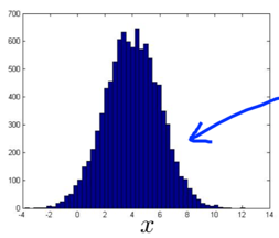
If the data doesn’t look like Gaussian, use a transformation to make it look more Gaussian.

 

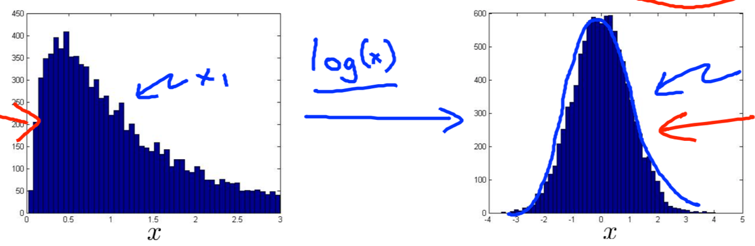
The algorithm usually works fine as well even if the data doesn’t look like Gaussian, but it might work better if the data does.

Common transformation: x:=log(x); x:=log(x)+c; x:=sqrt(x); x:=x^(1/c).

Problem: How to come up with features for an anomaly detection algorithm? 

Solution: Via an error analysis procedure.

Train an algorithm-> run the algorithm on cross validation set -> look at the examples it gets wrong, set if we can come up with extra features to improve.

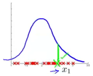
Common problem: p(x) are large for both normal and anomalous examples. But we want p(x) being large for normal examples and small for anomalous examples.

Solution: look at the wrongly flagged example(s) to see what went wrong, see if it can inspire us to come up with a new feature that help distinguish anomalous examples and other normal examples.

e.g. p(x1) is large for an anomalous example (in green) -> create new features x2.

How to choose features for anomaly detection

-> Create features that might take on unusually large or small values in the event of anomaly.

e.g. Monitoring computers in a data center

x1=memory usage; x2=number of disc accesses/sec; x3=CPU load; x4=network traffic.

Normally x3 and x4 grows linearly, but for an anomalous example, x3 grows but x4 doesn’t. -> create a new feature x5=x3/x4.

 

Multivariate Gaussian Distribution

1. Multivariate Gaussian Distribution

Problem: Sometimes anomaly detection algorithm fails to flag an anomaly example.

e.g. algorithm fails to detect the probability region (blue ellipse) thus p(x) for the anomaly example (green) is high.

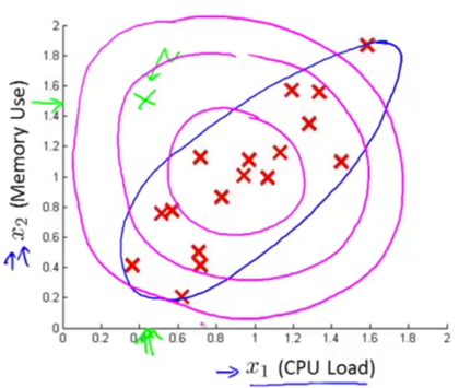
Solution: modified anomaly detection algorithm that uses multivariate Gaussian distribution (a.k.a. multivariate normal distribution).

multivariate Gaussian distribution: Model p(x) all in one go (x∈Rⁿ) instead of modeling p(x₁), p(x₂), … separately. 

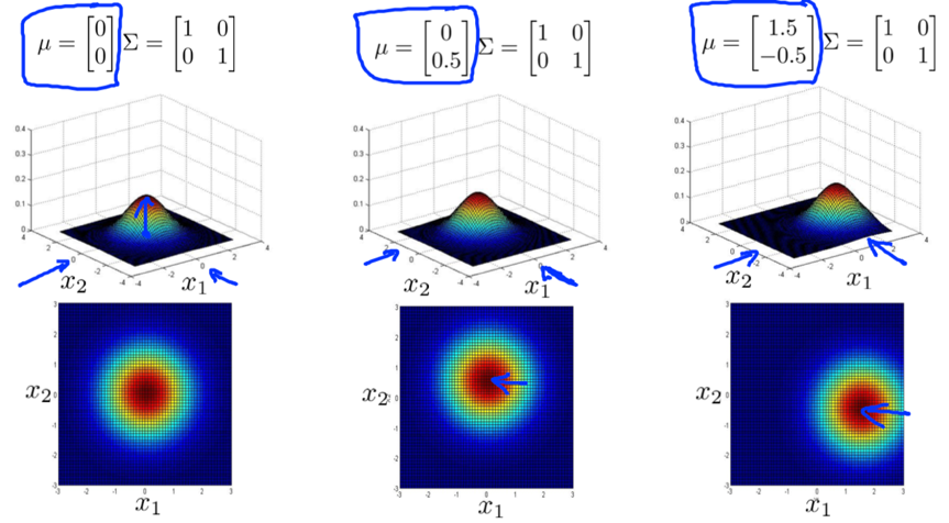
Parameters-> μ∈Rⁿ; ∑∈R^n*n. (μ: mean; ∑: covariance matrix).

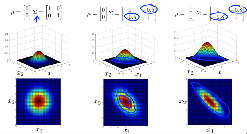
formula-> 

|∑| is the determinant of ∑, can be computed by det(sigma) in Octave.

e.g.

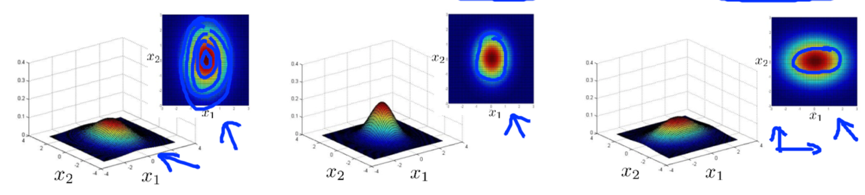
decrease/increase variance -> taller, narrower/wider, flatter distribution.

decrease/increase variance of one feature -> the distribution falls off more rapidly/slowly as that feature moves away.

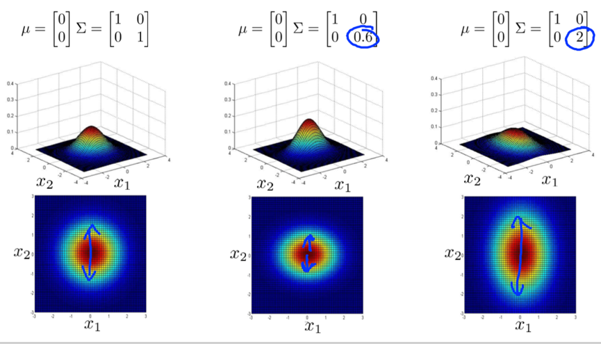
increase the positive value of off-diagonal entries of covariance->thinly peaked distribution along the x1=x2 line. (capture a positive correlation between x1 and x2)

increase the negative value of off-diagonal entries of covariance->thinly peaked distribution along the x1=-x2 line. (capture a negative correlation between x1 and x2)

vary mean-> shift the peak of the distribution

2. Anomaly Detection using the Multivariate Gaussian Distribution

Multivariate Gaussian Distribution:

Parameters-> μ∈Rⁿ; ∑∈R^n*n. (μ: mean; ∑: covariance matrix).

formula-> 

How to fit parameters:

Given training set {x⁽¹⁾, x⁽²⁾, …, x^(m)}, x∈Rⁿ,

formula->

Use multivariate Gaussian distribution in anomaly detection algorithm:

1) Take training set to fit model p(x) using the formula;

2) Given a new test example, compute p(x), flag it as anomaly if p(x)<ε.

Relationship between multivariate Gaussian distribution & the original model

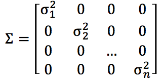
Original model: 

is a special case of multivariate Gaussian: 

with constraint that covariance ∑ must have 0s on all off-diagonal entries (thus the Gaussian are always axis-aligned).

e.g.

When to use original/multivariate Gaussian model

Original model: 

- Used more often.

- Need to create extra features if there’s unusual combinations of values. E.g. manually add feature x3=x1/x2.

- Computationally cheaper. Scales better to very large n (number of features).

- OK even if m (training set size) is small.

Multivariate Gaussian model:

- Used less often

- Better if you need to capture correlation of features because it can automatically capture correlations between different features.

- Computationally expensive, scales less well to large value of n.

- Must have m>n, or else ∑ is not invertible.

Rule of thumb: use multivariate Gaussian model only if m>=10n. 

If you find ∑ is singular when fitting multivariate Gaussian model:

Case 1: i m>n is not satisfied. -> Make sure m>n;

Case 2: there are redundant (linearly dependant) features. (e.g. x1=x2; x3=x4+5.) (though rarely happens) -> check and get rid of redundant features.

Recommender Systems

Predicting Movie Ratings

1. Problem Formulation

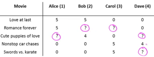
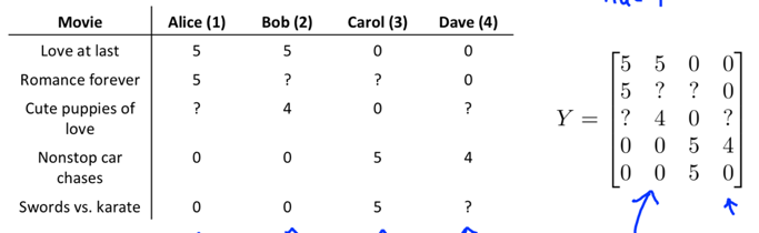
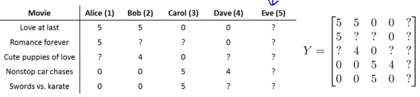
e.g. Given a set of movies and a set of users, each user has rated (0~5) some subset of movies->predict how they would have rated other movies they have not yet rated.

n_u=the number of users (4); n_m=the number of movies (5); 

r(i,j)=1 if user j has rated movie i;

y(i,j)=rating given by user j to movie i, defined only if r(i,j)=1.

Problem: Given dataset r(i,j) and y(i,j), predict what the unknown rating (?) should be.

Note: nu and nm written in superscript below are actually n_u and n_m instead of some product.

2. Content Based Recommendations

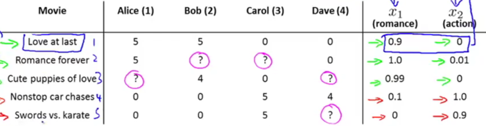
Given features x₁ and x₂, each movie can be represented with a feature vector (add feature x₀=1).

e.g. x(1)=[1, 0.9, 0]^T

-> treat predicting the ratings of each user as a separate linear regression problem

Problem formulation

Content based recommendations/approach: Assume we have features for the dataset, use these features of content to make prediction. 

r(i,j) = 1 if user j has rated movie i (0 otherwise)

y^(i,j)= rating by user j on movie i (if defined)

θ^(j)= parameter vector for user j, θ^(j)∈Rⁿ⁺¹, n=number of features (not counting x₀)

x⁽ⁱ⁾= feature vector for movie i.

m^(j)= number of movies rated by user j

n = number of features

-> For each user j, movie i, predict rating: (θ^(j))^Tx⁽ⁱ⁾

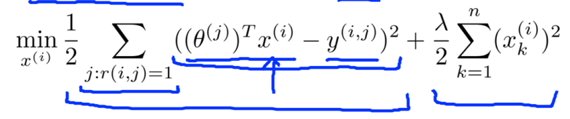
To learn θ^(j): 

* Given x⁽¹⁾, …, x^(nm), to learn θ⁽¹⁾, θ⁽²⁾, …,θ^(nu):

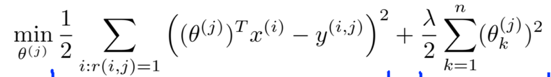
-> Optimization objective: J(θ⁽¹⁾, θ⁽²⁾, …, θ^(nu))

Optimization algorithm:

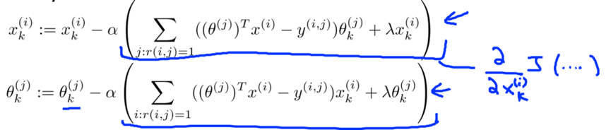
Gradient decent update: (essentially the same as linear regression except getting rid of 1/m^(j) term).

Difference between k=0 and k!=0 is because the θ₀ is not regularized in the optimization objective.

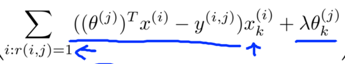  <-partial derivative with respect to parameters

Can also use another advanced optimization algorithm (e.g. conjugate gradient, LBFGS) to minimize J.

 

Collaborative Filtering

1. Collaborative Filtering – can learn for itself what features to use

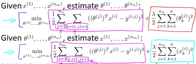
Given θ⁽¹⁾, …, θ^(nu) (users’preference), to learn x⁽ⁱ⁾ (feature vector for movie No.i): 

, y(i,j)=the rating of user j on movie i.

* Given θ⁽¹⁾, …, θ^(nu), to learn x⁽¹⁾, …, x^(nm): (learn features for all movies)

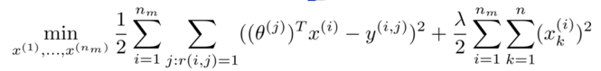
Collaborative filtering:

Difference:

Given features x⁽¹⁾, …, x^(nm) (and movie ratings), can estimate parameters θ⁽¹⁾, …, θ^(nu) (for different users).

v.s.

Given parameters θ⁽¹⁾, …, θ^(nu), can estimate features x⁽¹⁾, …, x^(nm) (for different movies).

Approach: (basic collaborative filtering algorithm)

-> randomly guess some value of θs, learn features x based on the initial θs;

-> get a better estimate of θs based on the initial x [by content based recommendations];

-> get a better estimate of x based on the new θs;

-> get θ->x->θ-> …back and forth until convergence.

2. Collaborative Filtering Algorithm

Problem: Go back and forth between guessing x and θ is less efficient.

 

Solution: An efficient algorithm that minimizes θ and x simultaneously. 

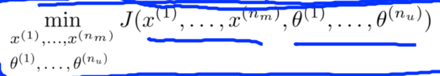
where J is a function of both x and θ:

 // The 1^st term equals to both the 1^st terms of the previous two cost function, and the following terms are just the regularization terms of the previous cost function.

Difference:

1) learn θ and x simultaneously instead of back and forth.

2) learn without the intercept term x₀=1 thus x, θ∈Rⁿ instead of Rⁿ⁺¹. (Therefore, there is no need to break out a special case to regularize θ₀ differently, either.)

Collaborative Filtering Algorithm

-> 1. Initialize x⁽¹⁾, …, x^(nm), θ⁽¹⁾, ..., θ^(nu) to small random values.

-> 2. Minimize cost function J(x⁽¹⁾, …, x^(nm), θ⁽¹⁾, ..., θ^(nu)) using gradient descent or some advanced optimization algorithm.

   e.g. for every j=1, …, n_u, i=1, …, n_m:

-> 3. Given a user with parameter θ and a movie with (learned) feature x, predict the rating as θ^Tx.

e.g. predict user j’s rating on movie i: (θ^(j))^T(x⁽ⁱ⁾).

 

Low Rank Matrix Factorization

1. Vectorization: Low Rank Matrix Factorization

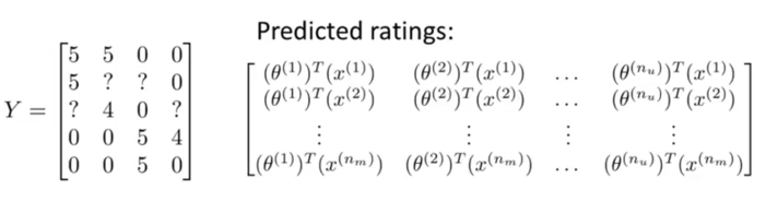
We can obtain a matrix of all predicted value by:

[Step 1] group the ranking data into a matrix. E.g. 

 [Step 2] Construct a matrix of predicted ratings where the (i,j) element (θ^(j))^T(x⁽ⁱ⁾) =user j’s predicted rating on movie i.

How to compute the matrix of predicted ratings in a vectorised way - low rank matrix factorization

Given ,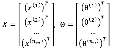

compute .

How to use the learned features to find related products

For each product (movies) i, we have learned a feature vector x⁽ⁱ⁾∈R;

-> Find a movie j that the distance ||x⁽ⁱ⁾-x^(j)|| is small.

e.g. To find 5 most similar movies to movies i

-> Find 5 movies j with the smallest  ||x⁽ⁱ⁾-x^(j)||.

2. Implementational Detail: Mean Normalization – can make the algorithm more efficient

Problem: If there are users who haven’t rated any movies/there are movies with no ratings.

Because the regularization term for θ is the only term in the cost function that effect J, collaborative learning will learn a θ=[0, …, 0]^T∈R^nu for that user (θ⁽⁵⁾ for Eve).

-> the prediction for that user on any movie i will be θx⁽ⁱ⁾=0, which will be unuseful.

Solution: Mean normalization.

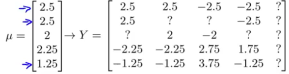
1) Compute the average rating that each movie obtained. (stored in vector μ)

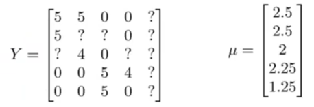
2) Subtract off the mean rating from the original rating. (so each movie will have an average rating of 0)

3) Use the new rating matrix as the dataset in collaborative learning algorithm to learn parameter θ and feature x.

4) For user j on movie i, prediction=(θ^(j))^T(x⁽ⁱ⁾)+μ_i.

For the user who haven’t rated any (5^th, Eve), its parameter (θ⁽⁵⁾) will still be [0, …, 0]^T,so prediction=(θ⁽⁵⁾)^T(x⁽ⁱ⁾)+μ_i= μ_i.

Large Scale Machine Learning

Gradient Descent with Large Datasets

1. Learning with Large Datasets

Problem: Batch gradient descent with large datasets comes with expensive computation -> Every iteration needs computing a derivative that sums over m (e.g. 100,000,000) examples.

A good sanity check: if training on a smaller random portion (e.g. 1000) of examples might do as well.

Checking method -> learning curve. 

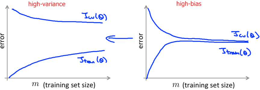
If the algorithm has high variance, then we know that adding more examples can improve.

If the algorithm has high bias, then we know that increasing m won’t improve much, better add extra features/hidden units (so that the learning curve would be changed to like the left one) before applying a large m.

2. Stochastic Gradient Descent

Stochastic gradient descent: a variant of batch gradient descent, scales better to much bigger training sets. Its idea can be applied to other learning algorithms that are based on training gradient descent on a specific training set (e.g. logistic regression, neural network) as well.

Stochastic gradient descent algorithm doesn’t need to look at all the training examples but only a single example in every iteration.

step of stochastic gradient descent

// Randomly shuffling the dataset ensures that we visit the training examples in a random order thus speed up the convergence.

1. Randomly shuffle (reorder) the dataset;

// Repeat time of the outer loop depends on the size of the training set, usually it’s enough to repeat the outer loop for 1~10 times.

2.

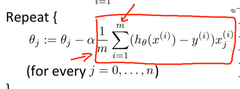
Repeat {
    for i:=1, …, m {
              
                (for every j := 0, 1, …, n)
    }
  }

Note that  is equal to  

What Stochastic gradient descent does is to scan through the training examples, modify the parameters just to fit one example better each time.

Stochastic gradient doesn’t actually converge in the same sense as Batch gradient descent does, but ends up wandering around continuously in some region close to the global minimum. (In practice, a parameter near the global minimum is usually good enough.)

3. Mini-Batch Gradient Descent

Mini-Batch Gradient Descent: Another variant of batch gradient descent, sometimes can work a bit faster than stochastic gradient descent.

Mini-Batch Gradient Descent is somewhere in between gradient descent and stochastic gradient descent.

Batch gradient descent: Use all m examples in each iteration.

Stochastic gradient descent: Use 1 example in each iteration.

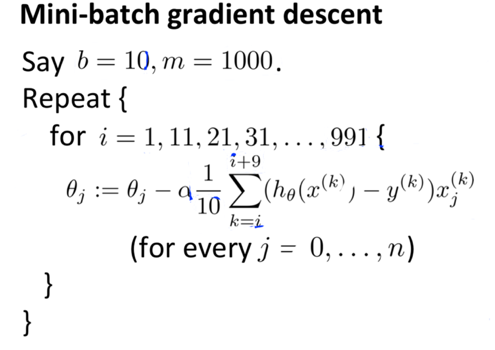
Mini-batch gradient descent: Use b examples in each iteration, where b is a parameter called “mini batch size”.

b is much smaller than m. typical choice: 10, typical range: 2~100.

i.e.  

-> get b examples (x⁽ⁱ⁾, y⁽ⁱ⁾), …, (x^(i+b-1), y^(i+b-1));

-> perform a gradient descent update using these b examples;

-> i:=i+b, go on to the next b examples and repeat.

Mini-batch gradient descent is

1) much faster than batch gradient descent.

2) likely to outperform Stochastic gradient descent if you have a good vectorised implementation. – by using good numerical algebra libraries that parallelize gradient computations over the b examples.

4. Stochastic Gradient Descent Convergence

How to debug (check the algorithm’s convergence)

Batch gradient descent (Review)

-> 

-> Plot J_train as a function of the number of iterations, make sure it is decreasing on every iteration.

With stochastic gradient descent, you don’t need to occasionally scan through the entire training set to compute J_train.

Stochastic gradient descent

-> 

-> During learning, compute cost(θ,(x⁽ⁱ⁾,y⁽ⁱ⁾)) before updating θusing (x⁽ⁱ⁾, y⁽ⁱ⁾). (compute how well the hypothesis is doing on that training example)

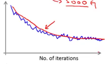
-> Every 1000 iterations, plot cost(θ,(x⁽ⁱ⁾,y⁽ⁱ⁾)) averaged over the last 1000 examples processed by the algorithm. (gives a running estimate of how well the algorithm is doing)

Plots of cost(θ,(x⁽ⁱ⁾,y⁽ⁱ⁾)) might look like

Because the plot of cost(θ,(x⁽ⁱ⁾,y⁽ⁱ⁾)) is averaged over 1000 examples, it might be noisy and doesn’t decrease on every single iteration.

The cost goes down then flatten out from some point->the algorithm has converged. (Blue)

If using a smaller learning rate, the cost will go down more slowly but might end up at a slightly better solution. (Red) Because stochastic gradient descent does not converge to the global minimum but oscillate a bit around the global minimum, it might end up with a smaller oscillation with a smaller learning rate.

 Increasing the number of examples to average over for every iteration (e.g. 1000->5000) makes the curve smoother, but the feedback you get on how well the algorithm is doing is more delayed. (Blue-1000; Red-5000.)

 If the plot is basically a flat curve, the cost might not be not decreasing at all. But it’s possible that the cost is actually decreasing, just that the original curve (Blue, average over 1000) is too noisy to see the actual trend. Averaging over a large number of examples (Red, average over 5000) might help.

i.e. If the plot is too noisy, try increasing the number of examples to average over to see the overall trend better.

If the curve is still flat even when averaging over a large number (magenta, average over 5000), the algorithm is really not learning much.

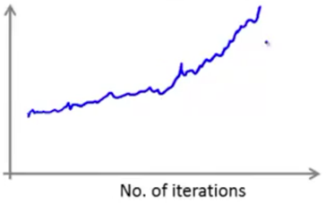
If the cost is increasing, it means that the algorithm is diverging, try using a smaller learning rate (α).

 

Learning rate

In most typical implementation of stochastic gradient descent, the learning rate α is held constant, so the contour plot ends up at like “the learned parameter will meander towards the minimum, wander around the global minimum forever but won’t really converge”.

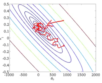
If you want stochastic gradient descent to actually converge at the global minimum, you can slowly decrease the learning rate αover time. 

E.g. 

iterationNumber - the number of iterations you’ve run of stochastic gradient descent;

const1, const2 – some constants as additional parameters of the algorithm that you might need to play with in order to get a good performance.

Cons: makes the algorithm more finicky because you need to spend time fiddle with 2 more extra parameters. (Thus typically people tend not to do this, keep the learning rate constant is more common.)

Pros: If you manage to tune the parameters well, as the algorithm gets closer toward the minimum when it meanders around, the meandering will get smaller and smaller until it hopefully converges to the global minimum.

 

Advanced Topics

1. Online Learning

Online Learning: Another large-scale learning setting that allows us to model problem where we have a continuous flood/stream of data coming in.

e.g. websites learn user preference from a continuous stream of data generated by users. 

e.g.

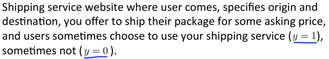
Goal: A learning algorithm to optimize appropriate prices as new users come to us.

-> Feature x: capture properties of users. E.g. the origin, the destination, the price we offer.

-> want:

    1) learn p(y=1|x;θ) --the probability that they will agree to use our shipping service given feature x.

    2) pick up a price that have a high probability (of choosing our service) while simultaneously offering us a fair profit.

Model p(y=1|x;θ) with logistic regression

We can use logistic regression, neural network or some other algorithm to model p(y=1|x;θ).

An online learning algorithm will:

Repeat forever { //because the website will keep on staying up
    Get (x,y) corresponding to user //Occasionally, a user comes
    Update θ using (x,y):
      --i.e. θj := θj-α(hθ(x)-y), for j=0, …, n
}

Notice: In other learning algorithm, we would update θusing (x⁽ⁱ⁾,y⁽ⁱ⁾), but for online learning we discard an example (x,y) after learning from it, there’s no need to number them.

i.e. look at one example at a time -> learn from that example -> discard it.

When to use online learning

-- When you have a continuous stream of users coming (data). Because data is unlimited so there’s no need to look at an example more than once.

If you have only a small number of users, better still saving all data in a fixed training set and run some algorithm over that set.

An advantage: Online learning algorithm can adapt to changing user preferences.

-- Because if the pool of users changes, the update of θ will slowly adapt the parameters to whatever the latest pool of users looks like. 

Other online learning applications

e.g. Product search problem: learn to give good product search listings to users

Users come to online cell-phone store website, type in query (e.g. “Android phone 1080p camera”) to search. Suppose we have 100 phones in store and will return 10 results in response to a search.

-> given the query, for each phone construct feature vector x that capture properties of the phone, how many words in the query match name of the phone, how many words in the query match description of the phone, etc.

-> suppose y=1 if user clicks on the link, y=0 otherwise.

-> Learn p(y=1|x;θ). A.k.a. learn the predict CTR (click-through rate).

-> Use the predicted CTR to show users the 10 phones they are most likely to click on.

Note: “we have 100 phones in store and will return 10 results in response to a search.” --> gives us 10 training examples (x, y) each time.

Other examples: choose special offers to show users; customized selection of news articles; product recommendation; … .

If you have a collaborative filtering system, you can use it to get additional features to feed into this logistic regression classifier.

Any of these problems could also have been formulated into as a standard machine learning problem (which has a fixed training set to run algorithm on), but in practice it’s better for large websites that get so much data to learn continuously through online learning than to save a fixed training set.

2. Map Reduce and Data Parallelism- A different approach to large scale machine learning

Maps reduce sometimes are more efficient than stochastic gradient descent for large problems.

Map reduce: 

1. Split the training set into multiple subsets, send them to different computers;

2. Each machine computes a summation of a portion instead of all m examples;

3. Computers send their result to a centralized server.

4. The centralized server combines the result together. -- The result is exactly equivalent to the batch gradient descent algorithm, only that the work load is divided up on multiple machines.

 

e.g. apply map reduce to batch gradient descent problems with m=400 (In practice, m will be much larger.) and 4 computers.

Batch gradient descent: 

-> Split the training set {(x⁽¹⁾,y⁽¹⁾), …, (x⁽⁴⁰⁰⁾,y⁽⁴⁰⁰⁾)} into several (e.g. 4) subsets;

-> let each machine compute that summation over some fraction of the training data;

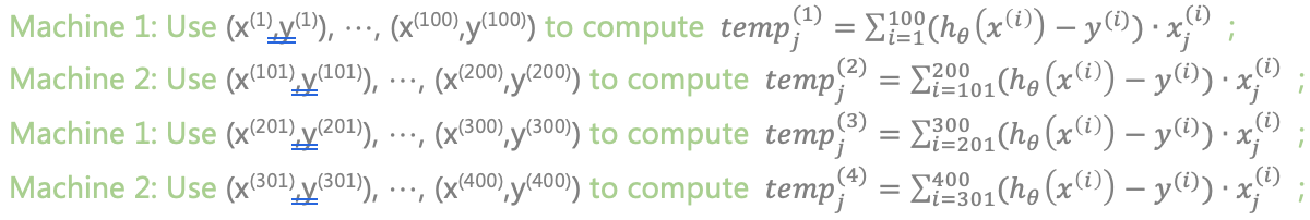
-> Send resulting temp variables to the centralized master server so it can combine them together to update the parameter:

, j=0, …,n.  

When can you apply map reduce to a learning algorithm to speed it up?

If your learning algorithm can be expressed as a summation over the training set, then map-reduce can be a good candidate for scaling your algorithm to large data sets.

Map reduce technique can be applied to other learning algorithms. e.g. Apply map reduce to logistic regression algorithm.

Need to compute: 1) Cost function of the optimization objective; 2) Partial derivatives. 

(They all can expressed as sums over the training set)

-> Split the training set into multiple subsets;

-> let each machine compute that summation over some fraction of the training data;

-> Machines send their results to a centralized server;

-> The server sums up all temp_j⁽ⁱ⁾to get the overall cost function and the overall partial derivatives (which can then be passed to the advanced optimization algorithm).

Map reduce can also be applied to a single computer with multiple cores.

-- By split the training set into multiple subsets and send them to different cores within the same single computer, divide up the workload, etc.

In this way network latency becomes a much less of an issue compared to parallelism over different computers, too.

Certain linear algebra libraries can automatically parallelize linear algebra operations across multiple cores within the machine. (Doesn’t apply to all libraries though.)

-- If you happen to be using one of those libraries and also have a good vectorising implementation of the learning algorithm, sometimes you can just implement a standard learning algorithm in a vectorised fashion without worrying about parallelization (i.e. implement map reduce), the library would take care of it.

Application Example: Photo OCR

1. Problem Description

Photo OCR (Optical Character Recognition) problem: to let computers find transcription of the text appears in the image.

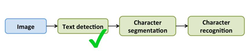
Photo OCR pipeline  -- an example of machine learning pipeline

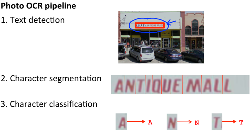
1) Text detection: Go through the image, find the region in the image where there’s text;

2) Character segmentation: Segment the given text region into the locations of individual characters;

3) Character classification: Recognize each individual character. – can apply a standard supervised learning (such as neural network) to do the multiclass classification, take an input image and classify what is the alphabet/digit character that appears in the image.

Some photo OCR system will also do spelling correction at the end, e.g. c1eaning->cleaning.

2. Sliding Windows-- How the sliding window classifier works in each individual components of Photo OCR pipeline

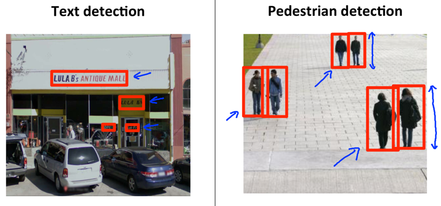
A simpler example: Pedestrian Detection – find each individual pedestrian appears in the image

construct a pedestrian detection system -- Train a supervised learning classifier using a sliding window detector

Although the heights of rectangles can be different depending on the pedestrian’s distance from the camera, their aspect ratio are the same.

-> Set x=pixels in 82*36 image patches //set the standard aspect ratio to 82*36

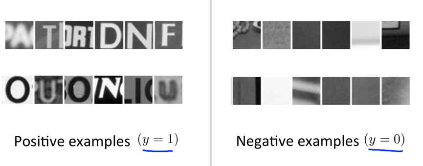
-> Collect a large (e.g. 1000~10000 examples) training set of positive and negative examples;

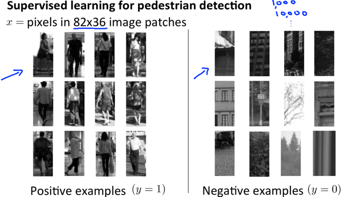
Goal: to train a (supervised) learning algorithm (e.g. neural network) that takes an 82*36 image patch as input and classifies whether or not a pedestrian appears in that image.

To detect pedestrians on a test set image:

-> Take a rectangular (e.g. 82*36) patch of the image

-> run that image patch through the classifier to decide whether a pedestrian appears in that image patch; 

-> Slide the rectangle over a bit, then run the new image patch through the classifier;

-> Slide the rectangle further, then run the new image patch through the classifier again;

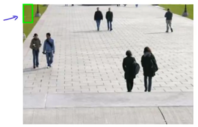
step size: a.k.a. stride, a parameter that is the amount you shift the rectangle over each time. Stride=1 (slide 1 pixel each time) usually performs best but is more computationally expensive.

-> start from another row after finishing shifting over the current row;

-> … 

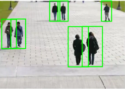
-> start with a larger window, use it to take larger image patches and run them through the classifier as well;

When taking larger image patches, resize them down to standard size (82*36) so that they can be passed through the classifier.

-> Can also do with even larger window, ….

-> Finally, the algorithm hopefully will be able to detect pedestrians.

sliding window for text detection:

Depending on the length of the text, the target rectangle regions can have different ratios.

-> Collect a labelled training set with positive examples (where there is text) and negative examples (where there is no text);

 

To detect text on a test set image:

To simplify, in this example we’ll going to run the sliding window classifier on just 1 fixed scale (i.e. rectangle size). 

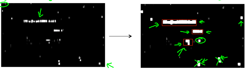
-> After running the sliding window classifier on lots of image patches, obtain an output image where white region means the classifier think it has found text there while different shades of grey correspond to the probabilities the classifier think it might have found text;

bright white -- very high estimated probability of there being text; darker region – lower probability.

-> apply an expansion operator to the output image which expands each of the white region a little bit;

   Implementation details: For every pixel, ask if it is within some distance (e.g. 5 pixels, 10 pixels.) of a white pixel in the output image (left), color that pixel as white in the new image (right) if it is true.

-> For the new image, rule out rectangles (using simple heuristic) whose aspect ratios that don’t look right (i.e. discard regions that are too tall and thin.), then draw bounding boxes around remaining continuous white regions.

-> Text detection is finished. Cut out image regions found and use later stage of pipeline to try to meet the texts.

Sliding window for character segmentation

Goal: To train a classifier (e.g. with neural network) to decide whether or not there is a split between 2 characters right in the middle using a labelled training set with positive (where the middle of the image represents a gap between 2 characters) and negative examples (where the middle of the image doesn’t represent the midpoint between 2 characters thus shouldn’t be split).

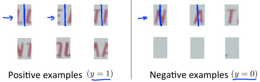
-> Run this trained classifier on a text region that the text detect system has pulled out:

  --> Start with a rectangle, ask the classifier whether or not we should put a split;

 

  --> Slide the window over, ask the classifier whether or not we should put a split;

(If the classifier output y=1, draw a line in the middle of the rectangle to split two characters.)

  --> Slide the window over again, …

  …

3. Getting Lots of Data and Artificial Data

Artificial Data Synthesis – an easy way to a huge training set for the learning algorithm.

Artificial data synthesis comprises of 2 main variations: 1) Creating new data from scratch; 2) Amplifying a small training set.

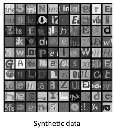
e.g. in character recognition

Creating new data from scratch – generate brand new data from scratch

-> We have already collected a labelled dataset of square image patches, by recognizing the character in the middle of each image patch, we have a small training set;

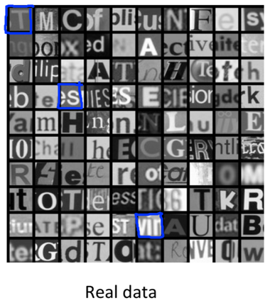
 -> Modern computers often have a huge font library, take characters from different fonts, and paste these characters against different random backgrounds;

 e.g. take a character ‘c’ from some font and paste it against a background, then we get a training example – an image of character ‘c’.

-> Can also apply a little blurring/distorting/shearing/scaling/rotation operations;

-> Eventually we get a synthetic training set:

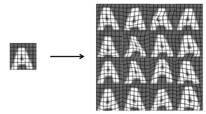
Amplifying a small training set – create additional data from existing data

-> Take an example image that we currently have, introduce artificial warping/artificial distortion into the image;

key: figure out what are reasonable sets ways to amplify/multiply the training set.

e.g. take a real image of character ‘A’ and warp it into 16 new examples:

e.g. For speech recognition application, amplify the training set by introducing different audio distortion:

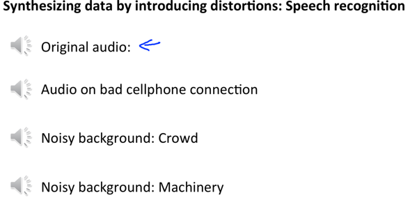
-> Eventually we amplify a small labelled training set to get a lot more examples.

Notice: The introduced distortion should be representative of the sorts of noise/distortion that you might see in the test set.

e.g. for character recognition, warping distortions are representative.

e.g. for speech recognition, bad cell phone connection/background noise are representative.

On the contrary, adding random/meaningless noise usually doesn’t help.

Advice

1. Before expending efforts on artificial data synthesize, make sure you really have a low biased classifier (sanity check, by plot learning curves) so that having more training data will be of help.

If you don’t have a low biased classifier, better keep increasing the number of features the classifier have or the number of hidden units in the neural network until you have a low biased classifier.

2. Always ask yourself/your team “how much work would it be to get 10x as much data as we currently have?”.

– sometimes you will be surprised how easy to greatly improve the product’s performance just from learning from a lot of data.

Ways to get a lot more data: 1) Artificial data synthesis; 2) Collect/label it yourself; 3) “Crown source”(hire people on internet inexpensively to label large training sets) e.g. Amazon Mechanical Turk.

 

4. Ceiling Analysis: What Part of the Pipeline to Work on Next

Problems: Sometimes developers spend a huge effort on improving a component but it actually doesn’t make a huge difference on performance of the final system.

Solution: Do a ceiling analysis to decide which part to improve rather than just trust a gut feeling.

Ceiling analysis gives a strong guidance on “what part of the pipeline might be the best use of your time to work on”.

As we go through the system giving more components the correct labels in the test set, the performance of the overall system goes up. We look at how much the performance goes up on different steps.

e.g. apply ceiling analysis on photo OCR pipeline

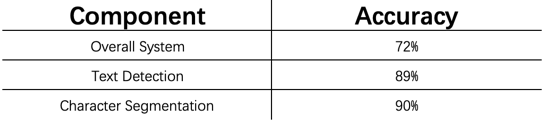
pre: better have a single rolled number evaluation metric for the learning system.

e.g. character level accuracy (the fraction of characters in the test set that are recognized correctly).

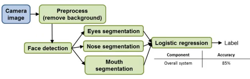
The accuracy of the overall system is 72%.

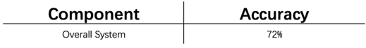
-> One module each time, manually provide it with the correct output of the test set, feed these ground true labels to the next stage of the pipeline.

E.g. For text detection module, manually label text area thus simulate a system with 100% accuracy in detecting text, then run through the rest of the pipeline (feed into character segmentation module) as usual.

with a simulated perfect text detection module, the overall system’s accuracy increases to 89%.

 

E.g. For the character segmentation module, give the test set the correct text detection output and character segmentation output.

…

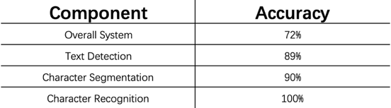
-> Get to know the upside potential of improving each of these components.

e.g. 

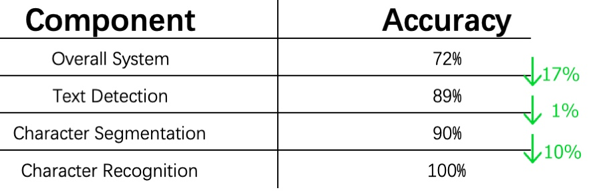
By getting perfect text detection, the performance goes from 72% to 89% (performance gain: 17%);

By getting perfect character segmentation, the performance goes from 89% to 90% (performance gain: only 1%, less worthy);

By getting perfect character recognition, the performance goes from 90% to 100% (performance gain: 10%).

e.g. apply ceiling analysis on face recognition – (this isn’t actually face recognition is done in practice)

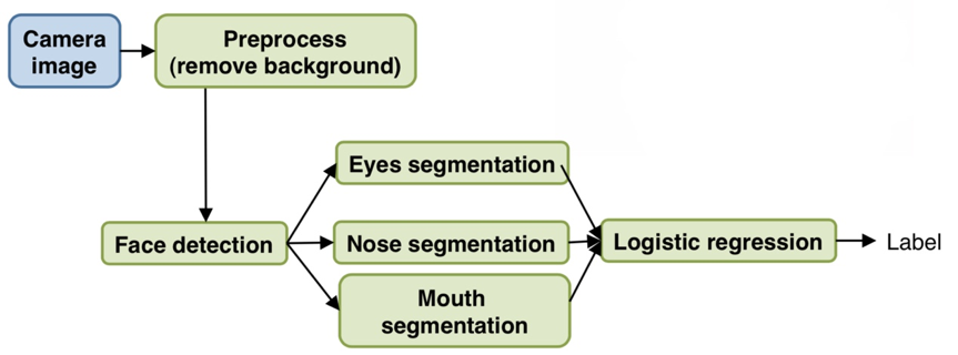
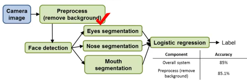
e.g. The overall system has 85% accuracy.

-> Go to the test set, manually remove the background, then we see that the accuracy goes up by 0.1%. (implying that background remove doesn’t worth a huge effort to work on.)

 

-> go to the test set, give it the correct face detection images, give correct locations of the eyes, …, etc, and finally give the correct overall label.

In the example, face detection component might be the most worthwhile working on (increase 5.9%).