机器学习 | 鸢尾花分类项目实战

前言：本系列博客参考于 《机器学习算法导论》和《Python机器学习》

如有侵权，敬请谅解。本书尽量用总结性的语言重述本书内容，避免侵权。

上一篇已经介绍了感知器算法规则，并且用 Python 语言实现了。现在我们应用感知器学习规则进行鸢尾花分类实验。

---

[QAQ ]

---

测试数据我们从鸢尾花数据集中挑选出了山鸢尾（Setosa）和变色鸢尾（Versicolor）两种花的信息作为测试数据。虽然感知器并不将数据样本特征的数量限定为两个，但出于可视化的原因，我们只考虑数据集中萼片长度（sepal length）和花瓣长度（petal length）这两个特征。同时，选择山鸢尾和变色鸢尾也是出于实践需要的考虑。不过，感知器算法可以扩展到多类别的分类器应用中，比如通过一对多技术。

注：一对多技术也称为一对其他技术，是一种将二分类技术扩充到多类别分类任务上的一种技术。

我们可以使用 (QvA) 针对每个类别训练一个分类器，其中分类器所对应类别样本为正类别，其他所有分类器的样本为负类别。

当应用与新数据样本识别时，我们可以借助于分类器 (phi(z)) ，其中m为类标数量，并将相关度最高的类标赋给待识别样本。对于感知器来说，就是最大净输入值绝对值对应的类标。

1、加载训练数据

使用 pandas 库直接从 (UCI) 机器学习库中将鸢尾花数据集转换为 DataFrame 对象并加载到内存中，并使用 tail 方法现实部分数据信息.

import pandas as pd

df = pd.read_csv(
    "https://archive.ics.uci.edu/ml/machine-learning-databases/iris/iris.data",
    header=None)
# df = pd.read_csv("iris.data", header=None)
# 输出最后20行的数据，并观察数据结构 萼片长度（sepal length），萼片宽度()，
# 花瓣长度（petal length），花瓣宽度，种类
print(df.tail(n=20))
print(df.shape)

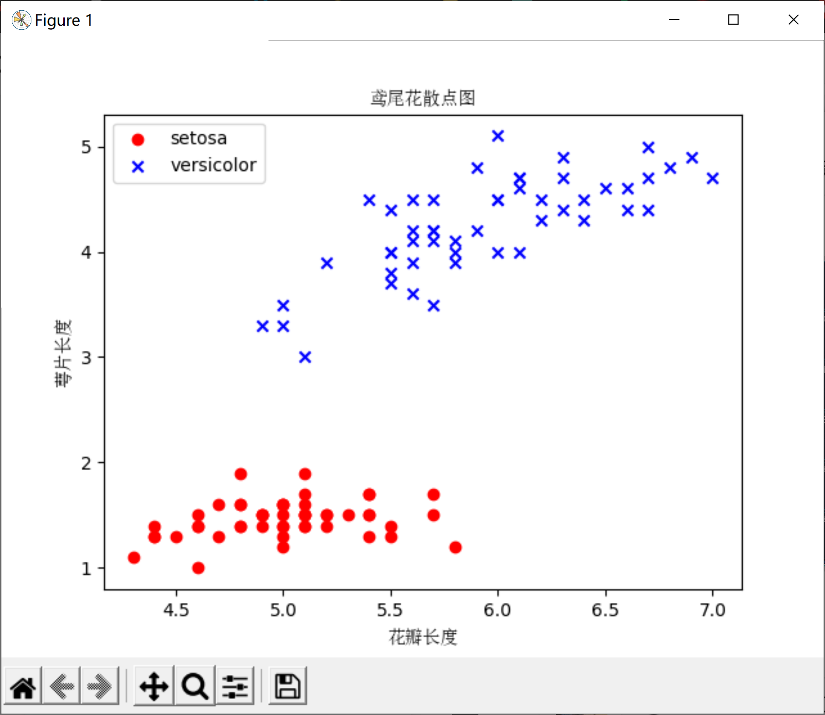
2、绘制训练数据

我们从鸢尾花数据集中提取前 (100) 个类标，其中分别包含 (50) 个山鸢尾类标和 (50) 个变色鸢尾类标，并将这些类标用两个整数值来替代：(1) 代表变色鸢尾，(-1) 代表山鸢尾，同时把 pandas DataFrame 产生的对应的整数类标赋值给 Numpy 的向量 (y)

类似的，我们提取这 (100) 个训练样本的第一个特征列（萼片长度）和第三个特征列（花瓣长度），并赋值给属性矩阵 (X)，这样我们就可以用二维散点图对这些数据进行可视化了。

# 0到100行，第5列
y = df.iloc[0:100, 4].values
# 将target值转数字化 Iris-setosa为-1，否则值为1
y = np.where(y == "Iris-setosa", -1, 1)
# 取出0到100行，第1，第三列的值
x = df.iloc[0:100, [0, 2]].values
""" 鸢尾花散点图 """

# scatter绘制点图
plt.scatter(x[0:50, 0], x[0:50, 1], color="red", marker="o", label="setosa")
plt.scatter(x[50:100, 0],
            x[50:100, 1],
            color="blue",
            marker="x",
            label="versicolor")
# 防止中文乱码 下面分别是windows系统，mac系统解决中文乱码方案
zh = mat.font_manager.FontProperties(fname='C:WindowsFontssimsun.ttc')
plt.title("鸢尾花散点图", fontproperties=zh)
plt.xlabel(u"花瓣长度", fontproperties=zh)
plt.ylabel(u"萼片长度", fontproperties=zh)
plt.legend(loc="upper left")
plt.show()

3、训练数据

现在我们可以利用抽取出的鸢尾花数据子集来训练感知器了。同时，我们还将绘制每次迭代的错误分类数量的折线图，以检验算法是否收敛并找到可以分开两种类型鸢尾花的决策边界。

训练代码：

from perceptron import Perceptron

import matplotlib.pyplot as plt
import matplotlib as mat
import pandas as pd
import numpy as np
"""
    训练模型并且记录错误次数，观察错误次数的变化
"""
print(__doc__)
# 加载鸢尾花数据
df = pd.read_csv(
    "https://archive.ics.uci.edu/ml/machine-learning-databases/iris/iris.data",
    header=None)
# df = pd.read_csv("iris.data", header=None)

# 数据真实值
y = df.iloc[0:100, 4].values
y = np.where(y == "Iris-setosa", -1, 1)
x = df.iloc[0:100, [0, 2]].values
"""
    误差数折线图 
    @:param eta: 0.1 学习速率
    @:param n_iter：0.1 迭代次数
"""
ppn = Perceptron(eta=0.1, n_iter=10)
ppn.fit(x, y)
# plot绘制折线图
plt.plot(range(1, len(ppn.errors_) + 1), ppn.errors_, marker="o")
# 防止中文乱码
zhfont1 = mat.font_manager.FontProperties(fname='C:WindowsFontssimsun.ttc')
plt.xlabel("迭代次数（n_iter）", fontproperties=zhfont1)
plt.ylabel("错误分类次数（error_number）", fontproperties=zhfont1)
plt.show()

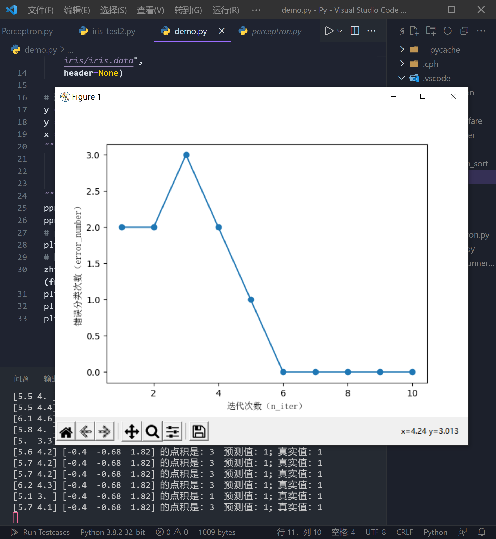
上面的代码绘制了每轮迭代的错误次数，从图可以看出，在第 (6) 轮迭代之后的出错次数已经降为 (0)（收敛），并且具备了对训练样本及进行正确分类的能力。

4、决策边界可视化

以下代码是对鸢尾花花萼长度、花瓣长度进行可视化及分类

from os import makedirs
import numpy as np
from sklearn import datasets
from sklearn.model_selection import train_test_split
from My_Perceptron import Perceptron
import matplotlib.pyplot as plt
import matplotlib as mat
import pandas as pd

iris = datasets.load_iris()
X = iris["data"][:, (0, 1)]
y = 2 * (iris["target"] == 0).astype(np.int64) - 1
X_train, X_test, y_train, y_test = train_test_split(X,
                                                    y,
                                                    test_size=0.4,
                                                    random_state=5)

model = Perceptron()
model.fit(X_train, y_train)
model.predict(X_test)

plt.figure(2)
plt.axis([4, 8, 1, 5])
plt.plot(X_train[:, 0][y_train == 1], X_train[:, 1][y_train == 1], "bs", ms=3)
plt.plot(X_train[:, 0][y_train == -1],
         X_train[:, 1][y_train == -1],
         "yo",
         ms=3)

x0 = np.linspace(4, 8, 200)
w = model.w
b = model.b
line = -w[0] / w[1] * x0 - b / w[1]
plt.plot(x0, line)

# 防止中文乱码 下面分别是windows系统，mac系统解决中文乱码方案
zh = mat.font_manager.FontProperties(fname='C:WindowsFontssimsun.ttc')
plt.title("鸢尾花散点图", fontproperties=zh)
plt.xlabel(u"花瓣长度", fontproperties=zh)
plt.ylabel(u"萼片长度", fontproperties=zh)
# plt.legend(loc="upper left")

plt.show()

---

import perceptron as pp
import pandas as pd
import matplotlib as mat

from matplotlib.colors import ListedColormap
import numpy as np
import matplotlib.pyplot as plt


def plot_decision_regions(x, y, classifier, resolution=0.2):
    """
    二维数据集决策边界可视化
    :parameter
    -----------------------------
    :param self: 将鸢尾花花萼长度、花瓣长度进行可视化及分类
    :param x: list 被分类的样本
    :param y: list 样本对应的真实分类
    :param classifier: method  分类器：感知器
    :param resolution:
    :return:
    -----------------------------
    """
    markers = ('s', 'x', 'o', '^', 'v')
    colors = ('red', 'blue', 'lightgreen', 'gray', 'cyan')
    # y去重之后的种类
    listedColormap = ListedColormap(colors[:len(np.unique(y))])

    # 花萼长度最小值-1，最大值+1
    x1_min, x1_max = x[:, 0].min() - 1, x[:, 0].max() + 1
    # 花瓣长度最小值-1，最大值+1
    x2_min, x2_max = x[:, 1].min() - 1, x[:, 1].max() + 1

    # 将最大值，最小值向量生成二维数组xx1,xx2
    # np.arange(x1_min, x1_max, resolution)  最小值最大值中间，步长为resolution
    new_x1 = np.arange(x1_min, x1_max, resolution)
    new_x2 = np.arange(x2_min, x2_max, resolution)
    xx1, xx2 = np.meshgrid(new_x1, new_x2)

    # 预测值
    # z = classifier.predict([xx1, xx2])
    z = classifier.predict(np.array([xx1.ravel(), xx2.ravel()]).T)
    z = z.reshape(xx1.shape)
    plt.contourf(xx1, xx2, z, alpha=0.4, camp=listedColormap)
    plt.xlim(xx1.min(), xx1.max())
    plt.ylim(xx2.min(), xx2.max())

    for idx, c1 in enumerate(np.unique(y)):
        plt.scatter(x=x[y == c1, 0],
                    y=x[y == c1, 1],
                    alpha=0.8,
                    c=listedColormap(idx),
                    marker=markers[idx],
                    label=c1)


df = pd.read_csv(
    "https://archive.ics.uci.edu/ml/machine-learning-databases/iris/iris.data",
    header=None)

# 0到100行，第5列
y = df.iloc[0:100, 4].values
# 将target值转数字化 Iris-setosa为-1，否则值为1,相当于激活函数-在此处表现为分段函数
y = np.where(y == "Iris-setosa", -1, 1)
# 取出0到100行，第1，第三列的值
x = df.iloc[0:100, [0, 2]].values
ppn = pp.Perceptron(eta=0.1, n_iter=10)
ppn.fit(x, y)
plot_decision_regions(x, y, classifier=ppn)
# 防止中文乱码
zhfont1 = mat.font_manager.FontProperties(fname='C:WindowsFontssimsun.ttc')
plt.title("鸢尾花花瓣、花萼边界分割", fontproperties=zhfont1)
plt.xlabel("花瓣长度 [cm]", fontproperties=zhfont1)
plt.ylabel("花萼长度 [cm]", fontproperties=zhfont1)

plt.legend(loc="uper left")
plt.show()