LeNet && ModernCNN

Convolutional Neural Networks

学而习之：Fundamentals of Convolutional Neural Networks

使用全连接层的局限性：

• 图像在同一列邻近的像素在这个向量中可能相距较远。它们构成的模式可能难以被模型识别。
• 对于大尺寸的输入图像，使用全连接层容易导致模型过大。

使用卷积层的优势：

• 卷积层保留输入形状。
• 卷积层通过滑动窗口将同一卷积核与不同位置的输入重复计算，从而避免参数尺寸过大。

卷积神经网络就是含卷积层的网络。

LeNet 模型

90%以上的参数都在全连接层块

LeNet分为卷积层块和全连接层块两个部分

解释：
    卷积层块由两个这样的基本单位重复堆叠构成。在卷积层块中，每个卷积层都使用$5 imes 5$的窗口，并在输出上使用sigmoid激活函数。第一个卷积层输出通道数为6，第二个卷积层输出通道数则增加到16。

    全连接层块含3个全连接层。它们的输出个数分别是120、84和10，其中10为输出的类别个数。

卷积层块里的基本单位

是卷积层后接平均池化层

卷积层用来识别图像里的空间模式，如线条和物体局部

之后的平均池化层则用来降低卷积层对位置的敏感性。

LeNet交替使用卷积层和最大池化层后接全连接层来进行图像分类

通过 Sequential 类实现 LeNet 模型

#import
import sys
sys.path.append("path to FashionMNIST2065")
import d2lzh1981 as d2l
import torch
import torch.nn as nn
import torch.optim as optim
import time

#net
class Flatten(torch.nn.Module):  #展平操作
    def forward(self, x):
        return x.view(x.shape[0], -1)

class Reshape(torch.nn.Module): #将图像大小重定型
    def forward(self, x):
        return x.view(-1,1,28,28)      #(B x C x H x W)

net = torch.nn.Sequential(     #Lelet                                                  
    Reshape(),  
    # 公式：[(nh-kh+ph+sh)/sh]*[(nw-kw+pw+sw)/sw]
    nn.Conv2d(in_channels=1, out_channels=6, kernel_size=5, padding=2), #b*1*28*28  =>b*6*28*28
    nn.Sigmoid(),     
    # 平均池化
    nn.AvgPool2d(kernel_size=2, stride=2),                     #b*6*28*28  =>b*6*14*14
    nn.Conv2d(in_channels=6, out_channels=16, kernel_size=5),  #b*6*14*14  =>b*16*10*10
    nn.Sigmoid(),
    nn.AvgPool2d(kernel_size=2, stride=2),                     #b*16*10*10  => b*16*5*5
    # 展平
    Flatten(),                                                 #b*16*5*5   => b*400
    # 三个全连接层
    nn.Linear(in_features=16*5*5, out_features=120),
    nn.Sigmoid(),
    nn.Linear(120, 84),
    nn.Sigmoid(),
    nn.Linear(84, 10)
)

获取数据

# 数据
batch_size = 256
train_iter, test_iter = d2l.load_data_fashion_mnist(
    batch_size=batch_size, root='path to FashionMNIST2065')
# 训练集批次数
print(len(train_iter))
'''
额外的数据表示，以图像形式显示
'''
#数据展示
import matplotlib.pyplot as plt
# define drawing function
def show_fashion_mnist(images, labels):
    d2l.use_svg_display()
    # 这里的_表示我们忽略（不使用）的变量
    _, figs = plt.subplots(1, len(images), figsize=(12, 12))
    for f, img, lbl in zip(figs, images, labels):
        f.imshow(img.view((28, 28)).numpy())
        f.set_title(lbl)
        f.axes.get_xaxis().set_visible(False)
        f.axes.get_yaxis().set_visible(False)
    plt.show()

for Xdata,ylabel in train_iter:
    break
X, y = [], []
for i in range(10):
    print(Xdata[i].shape,ylabel[i].numpy())
    X.append(Xdata[i]) # 将第i个feature加到X中
    y.append(ylabel[i].numpy()) # 将第i个label加到y中
show_fashion_mnist(X, y)

---

因为卷积神经网络计算比多层感知机要复杂，建议使用GPU来加速计算。我们查看看是否可以用GPU，如果成功则使用 cuda:0，否则仍然使用 cpu。

# This function has been saved in the d2l package for future use
#use GPU
def try_gpu():
    """If GPU is available, return torch.device as cuda:0; else return torch.device as cpu."""
    if torch.cuda.is_available():
        device = torch.device('cuda:0')
    else:
        device = torch.device('cpu')
    return device

device = try_gpu()
device

---

训练

计算准确率

'''
(1). net.train()
  启用 BatchNormalization 和 Dropout，将BatchNormalization和Dropout置为True
(2). net.eval()
不启用 BatchNormalization 和 Dropout，将BatchNormalization和Dropout置为False
'''
'''
:param:data_iter:测试集
:param:acc_sum:模型预测正确的总数
:param:n:预测总数
'''
def evaluate_accuracy(data_iter, net,device=torch.device('cpu')):
    """Evaluate accuracy of a model on the given data set."""
    acc_sum,n = torch.tensor([0],dtype=torch.float32,device=device),0
    for X,y in data_iter:
        # If device is the GPU, copy the data to the GPU.
        # 把tensorc传到device中
        X,y = X.to(device),y.to(device)
        # 网络正在进行预测
        net.eval()
        该区域涉及到的数据不需要计算梯度，也不进行反向传播
        with torch.no_grad():
            y = y.long()
            # 将一个批次的训练数据X通过网络模型net输出
            # 经过argmax得到预测值
            # dim维度选择为1
            acc_sum += torch.sum((torch.argmax(net(X), dim=1) == y))  #[[0.2 ,0.4 ,0.5 ,0.6 ,0.8] ,[ 0.1,0.2 ,0.4 ,0.3 ,0.1]] => [ 4 , 2 ]
            # 预测的总数相加
            n += y.shape[0]
    # 预测准确率
    return acc_sum.item()/n

训练函数

#训练函数
def train_ch5(net, train_iter, test_iter,criterion, num_epochs, batch_size, device,lr=None):
    """Train and evaluate a model with CPU or GPU."""
    print('training on', device)
    net.to(device)
    optimizer = optim.SGD(net.parameters(), lr=lr)
    for epoch in range(num_epochs):
        train_l_sum = torch.tensor([0.0],dtype=torch.float32,device=device)
        train_acc_sum = torch.tensor([0.0],dtype=torch.float32,device=device)
        n, start = 0, time.time()
        for X, y in train_iter:
            net.train()
            # 梯度清零 不同批次的梯度不相关
            optimizer.zero_grad()
            X,y = X.to(device),y.to(device) 
            # 预测值
            y_hat = net(X)
            loss = criterion(y_hat, y)
            # 梯度回传
            loss.backward()
            optimizer.step()
            
            with torch.no_grad():
                y = y.long()
                train_l_sum += loss.float()
                # 训练集中预测正确的总数
                train_acc_sum += (torch.sum((torch.argmax(y_hat, dim=1) == y))).float()
                n += y.shape[0]
        test_acc = evaluate_accuracy(test_iter, net,device)
        print('epoch %d, loss %.4f, train acc %.3f, test acc %.3f, '
              'time %.1f sec'
              % (epoch + 1, train_l_sum/n, train_acc_sum/n, test_acc,
                 time.time() - start))

训练进程

模型参数初始化到 device 中，并使用 Xavier 随机初始化。损失函数和训练算法则依然使用交叉熵损失函数和小批量随机梯度下降。

Xavier 随机初始化 —参考学而后思,方能发展;思而立行,终将卓越

# 训练 学习率0.9
lr, num_epochs = 0.9, 10

def init_weights(m):
    if type(m) == nn.Linear or type(m) == nn.Conv2d:
        torch.nn.init.xavier_uniform_(m.weight)

net.apply(init_weights)
net = net.to(device)

criterion = nn.CrossEntropyLoss()   #交叉熵描述了两个概率分布之间的距离，交叉熵越小说明两者之间越接近
train_ch5(net, train_iter, test_iter, criterion,num_epochs, batch_size,device, lr)

测试

# test
for testdata,testlabe in test_iter:
    testdata,testlabe = testdata.to(device),testlabe.to(device)
    break
print(testdata.shape,testlabe.shape)
net.eval()
y_pre = net(testdata)
# 预测值
print(torch.argmax(y_pre,dim=1)[:10])
# 真实标签
print(testlabe[:10])

深度卷积神经网络（AlexNet）

2014年ImgNet竞赛中

证明了学习到的特征可以超过手工设计的特征, 打破计算机视觉研究的前状

知缺陷方能进步

LeNet: 在大的真实数据集上的表现并不尽如⼈意。

1.神经网络计算复杂。

2.还没有⼤量深⼊研究参数初始化和⾮凸优化算法等诸多领域。

在此之后，针对特征的选择分为两派：

• 机器学习的特征提取:手工定义的特征提取函数
• 神经网络的特征提取：通过学习得到数据的多级表征，并逐级表⽰越来越抽象的概念或模式。

神经网络发展的限制:数据、硬件

AlexNet

设计理念核Lenet相似

特征：

1. 8层变换，其中有5层卷积和2层全连接隐藏层，以及1个全连接输出层。
2. 将sigmoid激活函数改成了更加简单的ReLU激活函数。
3. 用Dropout来控制全连接层的模型复杂度。
4. 引入数据增强，如翻转、裁剪和颜色变化，从而进一步扩大数据集来缓解泛化能力不好导致的过拟合。

$数据集.MINIST(Left) IMAGENET(Right)$

利用padding 的作用：使得输入和输出的形状相同

可以参考 Fundamentals of Convolutional Neural Networks

import time
import torch
from torch import nn, optim
import torchvision
import numpy as np
import sys
sys.path.append("path to FashionMNIST2065") 
import d2lzh1981 as d2l
import os
import torch.nn.functional as F

device = torch.device('cuda' if torch.cuda.is_available() else 'cpu')

实现 AlexNet 模型

class AlexNet(nn.Module):
    def __init__(self):
        super(AlexNet, self).__init__()
        self.conv = nn.Sequential(
            # 默认不做padding
            nn.Conv2d(1, 96, 11, 4), # in_channels, out_channels, kernel_size, stride, padding
            nn.ReLU(),
            nn.MaxPool2d(3, 2), # kernel_size, stride
            # 减小卷积窗口，使用填充为2来使得输入与输出的高和宽一致，且增大输出通道数
            nn.Conv2d(96, 256, 5, 1, 2),
            nn.ReLU(),
            nn.MaxPool2d(3, 2),
            # 连续3个卷积层，且使用更小的卷积窗口。除了最后的卷积层外，进一步增大了输出通道数。
            # 前两个卷积层后不使用池化层来减小输入的高和宽
            nn.Conv2d(256, 384, 3, 1, 1),
            nn.ReLU(),
            nn.Conv2d(384, 384, 3, 1, 1),
            nn.ReLU(),
            nn.Conv2d(384, 256, 3, 1, 1),
            nn.ReLU(),
            nn.MaxPool2d(3, 2)
        )
        # 这里全连接层的输出个数比LeNet中的大数倍。使用丢弃层来缓解过拟合
        self.fc = nn.Sequential(
            nn.Linear(256*5*5, 4096),
            nn.ReLU(),
            nn.Dropout(0.5),
            #由于使用CPU镜像，精简网络，若为GPU镜像可添加该层
            #nn.Linear(4096, 4096),
            #nn.ReLU(),
            #nn.Dropout(0.5),

            # 输出层。由于这里使用Fashion-MNIST，所以用类别数为10，而非论文中的1000
            nn.Linear(4096, 10),
        )

    def forward(self, img):

        feature = self.conv(img)
        output = self.fc(feature.view(img.shape[0], -1))
        return output

载入数据

def load_data_fashion_mnist(batch_size, resize=None, root='/home/kesci/input/FashionMNIST2065'):
    """Download the fashion mnist dataset and then load into memory."""
    trans = []
    if resize:
        trans.append(torchvision.transforms.Resize(size=resize))
    trans.append(torchvision.transforms.ToTensor())
    
    transform = torchvision.transforms.Compose(trans)
    mnist_train = torchvision.datasets.FashionMNIST(root=root, train=True, download=True, transform=transform)
    mnist_test = torchvision.datasets.FashionMNIST(root=root, train=False, download=True, transform=transform)

    train_iter = torch.utils.data.DataLoader(mnist_train, batch_size=batch_size, shuffle=True, num_workers=2)
    test_iter = torch.utils.data.DataLoader(mnist_test, batch_size=batch_size, shuffle=False, num_workers=2)

    return train_iter, test_iter

#batchsize=128
batch_size = 16
# 如出现“out of memory”的报错信息，可减小batch_size或resize
train_iter, test_iter = load_data_fashion_mnist(batch_size,224)
for X, Y in train_iter:
    print('X =', X.shape,
        '
Y =', Y.type(torch.int32))
    break

训练

lr, num_epochs = 0.001, 3
optimizer = torch.optim.Adam(net.parameters(), lr=lr)
d2l.train_ch5(net, train_iter, test_iter, batch_size, optimizer, device, num_epochs)

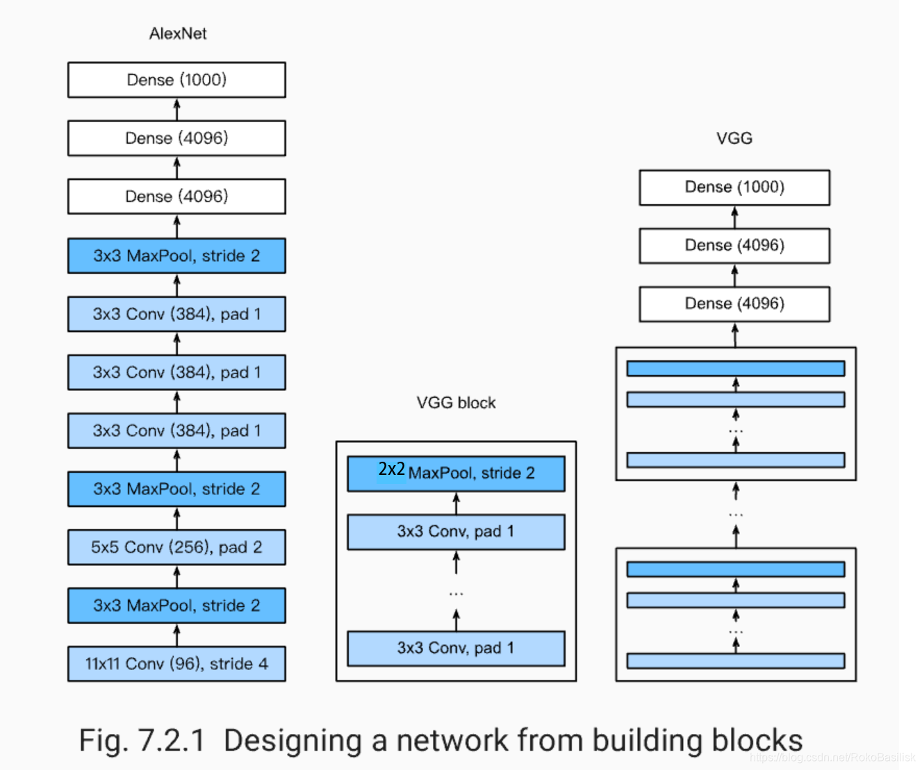
使用重复元素的网络（VGG）

知缺陷方能进步

AlxNet

并没有提供简单的规则来制造新的网络

结构比较死板

所以 VGG：通过重复使⽤简单的基础块来构建深度模型。

Block:数个相同的填充为1、窗口形状为$3 imes 3$的卷积层,接上一个步幅为2、窗口形状为$2 imes 2$的最大池化层。

卷积层保持输入的高和宽不变，而池化层则对其减半

VGG11的实现

# 可以修改的参数 e每个vgg_block结构相同但是参数可能不相同
def vgg_block(num_convs, in_channels, out_channels): #卷积层个数，输入通道数，输出通道数
    blk = []
    for i in range(num_convs):
        if i == 0:
            blk.append(nn.Conv2d(in_channels, out_channels, kernel_size=3, padding=1))
        else:
            blk.append(nn.Conv2d(out_channels, out_channels, kernel_size=3, padding=1))
        blk.append(nn.ReLU())
    blk.append(nn.MaxPool2d(kernel_size=2, stride=2)) # 这里会使宽高减半
    return nn.Sequential(*blk)
conv_arch = ((1, 1, 64), (1, 64, 128), (2, 128, 256), (2, 256, 512), (2, 512, 512))
# 经过5个vgg_block, 宽高会减半5次, 变成 224/32 = 7
fc_features = 512 * 7 * 7 # c * w * h
fc_hidden_units = 4096 # 任意

# vgg模型
def vgg(conv_arch, fc_features, fc_hidden_units=4096):
    net = nn.Sequential()
    # 卷积层部分
    for i, (num_convs, in_channels, out_channels) in enumerate(conv_arch):
        # 每经过一个vgg_block都会使宽高减半
        net.add_module("vgg_block_" + str(i+1), vgg_block(num_convs, in_channels, out_channels))
    # 全连接层部分
    net.add_module("fc", nn.Sequential(d2l.FlattenLayer(),
                                 nn.Linear(fc_features, fc_hidden_units),
                                 nn.ReLU(),
                                 nn.Dropout(0.5),
                                 nn.Linear(fc_hidden_units, fc_hidden_units),
                                 nn.ReLU(),
                                 nn.Dropout(0.5),
                                 nn.Linear(fc_hidden_units, 10)
                                ))
    return net

net = vgg(conv_arch, fc_features, fc_hidden_units)
X = torch.rand(1, 1, 224, 224)

# named_children获取一级子模块及其名字(named_modules会返回所有子模块,包括子模块的子模块)
for name, blk in net.named_children(): 
    X = blk(X)
    print(name, 'output shape: ', X.shape)
ratio = 8
# 减小vgg结构，针对minist数据集较小，数据少参数多容易造成过拟合
small_conv_arch = [(1, 1, 64//ratio), (1, 64//ratio, 128//ratio), (2, 128//ratio, 256//ratio), 
                   (2, 256//ratio, 512//ratio), (2, 512//ratio, 512//ratio)]
net = vgg(small_conv_arch, fc_features // ratio, fc_hidden_units // ratio)
print(net)

batchsize=16
#batch_size = 64
# 如出现“out of memory”的报错信息，可减小batch_size或resize
# train_iter, test_iter = d2l.load_data_fashion_mnist(batch_size, resize=224)

lr, num_epochs = 0.001, 5
optimizer = torch.optim.Adam(net.parameters(), lr=lr)
d2l.train_ch5(net, train_iter, test_iter, batch_size, optimizer, device, num_epochs)

网络中的网络（NiN）

知缺陷方能进步

LeNet、AlexNet和VGG

先以由卷积层构成的模块充分抽取 空间特征

再以由全连接层构成的模块来输出分类结果

NiN

串联多个由卷积层和 “全连接” 层构成的小⽹络来构建⼀个深层⽹络。

NiN去掉了全连接层，而是用平均池化层

⽤了输出通道数等于标签类别数的NiN块，然后使⽤全局平均池化层对每个通道中所有元素求平均并直接⽤于分类。 这样的设计显著的减少了参数尺寸防止过拟合，但是增加了训练时间

---

$1 imes1$卷积核作用:

1. 放缩通道数：通过控制卷积核的数量达到通道数的放缩。
2. 增加非线性。1×1卷积核的卷积过程相当于全连接层的计算过程，并且还加入了非线性激活函数，从而可以增加网络的非线性。
3. 计算参数少

---

NiN 的实现

# 构建组成模块nin_block
def nin_block(in_channels, out_channels, kernel_size, stride, padding):
    blk = nn.Sequential(nn.Conv2d(in_channels, out_channels, kernel_size, stride, padding),
                        nn.ReLU(),
                        nn.Conv2d(out_channels, out_channels, kernel_size=1),
                        nn.ReLU(),
                        nn.Conv2d(out_channels, out_channels, kernel_size=1),
                        nn.ReLU())
    return blk

class GlobalAvgPool2d(nn.Module):
    # 全局平均池化层可通过将池化窗口形状设置成输入的高和宽实现
    def __init__(self):
        super(GlobalAvgPool2d, self).__init__()
    def forward(self, x):
        return F.avg_pool2d(x, kernel_size=x.size()[2:])

net = nn.Sequential(
    nin_block(1, 96, kernel_size=11, stride=4, padding=0),
    nn.MaxPool2d(kernel_size=3, stride=2),
    nin_block(96, 256, kernel_size=5, stride=1, padding=2),
    nn.MaxPool2d(kernel_size=3, stride=2),
    nin_block(256, 384, kernel_size=3, stride=1, padding=1),
    nn.MaxPool2d(kernel_size=3, stride=2), 
    nn.Dropout(0.5),
    # 标签类别数是10
    nin_block(384, 10, kernel_size=3, stride=1, padding=1),
    GlobalAvgPool2d(), 
    # 将四维的输出转成二维的输出，其形状为(批量大小, 10)
    d2l.FlattenLayer())

batch_size = 128
# 如出现“out of memory”的报错信息，可减小batch_size或resize
#train_iter, test_iter = d2l.load_data_fashion_mnist(batch_size, resize=224)

lr, num_epochs = 0.002, 5
optimizer = torch.optim.Adam(net.parameters(), lr=lr)
d2l.train_ch5(net, train_iter, test_iter, batch_size, optimizer, device, num_epochs)

NiN

• NiN重复使⽤由卷积层和代替全连接层的1×1卷积层构成的NiN块来构建深层⽹络 ;
• NiN去除了容易造成过拟合的全连接输出层，而是将其替换成输出通道数等于标签类别数 的NiN块和全局平均池化层 ;
• NiN的以上设计思想影响了后⾯⼀系列卷积神经⽹络的设计 ;

GoogLeNet

牺牲了串联网络的思想

1. 由 Inception 基础块组成。
2. Inception 块相当于⼀个有4条线路的⼦⽹络。它通过不同窗口形状的卷积层和最⼤池化层来并⾏抽取信息，并使⽤1×1卷积层减少通道数从而降低模型复杂度。
3. 可以⾃定义的超参数是每个层的输出通道数，我们以此来控制模型复杂度。
4. 使用 padding 来保证输入输出形状相同
   

Inception 基础块实现

class Inception(nn.Module):
    # c1 - c4为每条线路里的层的输出通道数
    def __init__(self, in_c, c1, c2, c3, c4):
        super(Inception, self).__init__()
        # 线路1，单1 x 1卷积层
        self.p1_1 = nn.Conv2d(in_c, c1, kernel_size=1)
        # 线路2，1 x 1卷积层后接3 x 3卷积层
        self.p2_1 = nn.Conv2d(in_c, c2[0], kernel_size=1)
        self.p2_2 = nn.Conv2d(c2[0], c2[1], kernel_size=3, padding=1)
        # 线路3，1 x 1卷积层后接5 x 5卷积层
        self.p3_1 = nn.Conv2d(in_c, c3[0], kernel_size=1)
        self.p3_2 = nn.Conv2d(c3[0], c3[1], kernel_size=5, padding=2)
        # 线路4，3 x 3最大池化层后接1 x 1卷积层
        self.p4_1 = nn.MaxPool2d(kernel_size=3, stride=1, padding=1)
        self.p4_2 = nn.Conv2d(in_c, c4, kernel_size=1)

    def forward(self, x):
        p1 = F.relu(self.p1_1(x))
        p2 = F.relu(self.p2_2(F.relu(self.p2_1(x))))
        p3 = F.relu(self.p3_2(F.relu(self.p3_1(x))))
        p4 = F.relu(self.p4_2(self.p4_1(x)))
        return torch.cat((p1, p2, p3, p4), dim=1)  # 在通道维上连结输出

完整模型结构

$input -1 imes96 imes96$

# 抽取特征来减小大小
b1 = nn.Sequential(nn.Conv2d(1, 64, kernel_size=7, stride=2, padding=3),
                   nn.ReLU(),
                   nn.MaxPool2d(kernel_size=3, stride=2, padding=1))

b2 = nn.Sequential(nn.Conv2d(64, 64, kernel_size=1),
                   nn.Conv2d(64, 192, kernel_size=3, padding=1),
                   nn.MaxPool2d(kernel_size=3, stride=2, padding=1))

b3 = nn.Sequential(Inception(192, 64, (96, 128), (16, 32), 32),
                   Inception(256, 128, (128, 192), (32, 96), 64),
                   nn.MaxPool2d(kernel_size=3, stride=2, padding=1))

b4 = nn.Sequential(Inception(480, 192, (96, 208), (16, 48), 64),
                   Inception(512, 160, (112, 224), (24, 64), 64),
                   Inception(512, 128, (128, 256), (24, 64), 64),
                   Inception(512, 112, (144, 288), (32, 64), 64),
                   Inception(528, 256, (160, 320), (32, 128), 128),
                   nn.MaxPool2d(kernel_size=3, stride=2, padding=1))

b5 = nn.Sequential(Inception(832, 256, (160, 320), (32, 128), 128),
                   Inception(832, 384, (192, 384), (48, 128), 128),
                   d2l.GlobalAvgPool2d())

net = nn.Sequential(b1, b2, b3, b4, b5, 
                    d2l.FlattenLayer(), nn.Linear(1024, 10))

net = nn.Sequential(b1, b2, b3, b4, b5, d2l.FlattenLayer(), nn.Linear(1024, 10))

X = torch.rand(1, 1, 96, 96)

for blk in net.children(): 
    X = blk(X)
    print('output shape: ', X.shape)

#batchsize=128
batch_size = 16
# 如出现“out of memory”的报错信息，可减小batch_size或resize
#train_iter, test_iter = d2l.load_data_fashion_mnist(batch_size, resize=96)

lr, num_epochs = 0.001, 5
optimizer = torch.optim.Adam(net.parameters(), lr=lr)
d2l.train_ch5(net, train_iter, test_iter, batch_size, optimizer, device, num_epochs)