视频实时换脸明星动画—最新案例
1、演示视频案例一
下边为原主播
其次,进行实时变脸,依次为刘亦菲、唐嫣、杨幂、范冰冰
Ref:https://blog.csdn.net/qq_41185868/article/details/81047974
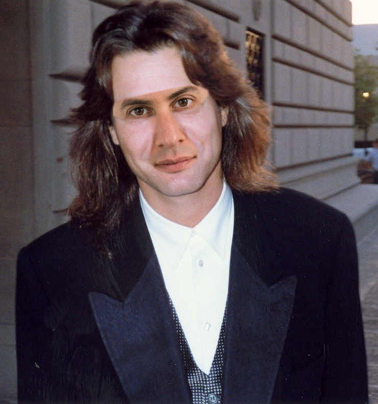
Switching Eds: Face swapping with Python, dlib, and OpenCV
Introduction
In this post I’ll describe how I wrote a short (200 line) Python script to automatically replace facial features on an image of a face, with the facial features from a second image of a face.
The process breaks down into four steps:
- Detecting facial landmarks.
- Rotating, scaling, and translating the second image to fit over the first.
- Adjusting the colour balance in the second image to match that of the first.
- Blending features from the second image on top of the first.
The full source-code for the script can be found here.
1. Using dlib to extract facial landmarks
The script uses dlib’s Python bindings to extract facial landmarks:

 1 PREDICTOR_PATH = "/home/matt/dlib-18.16/shape_predictor_68_face_landmarks.dat"
 2
 3 detector = dlib.get_frontal_face_detector()
 4 predictor = dlib.shape_predictor(PREDICTOR_PATH)
 5
 6 def get_landmarks(im):
 7     rects = detector(im, 1)
 8
 9     if len(rects) > 1:
10         raise TooManyFaces
11     if len(rects) == 0:
12         raise NoFaces
13
14     return numpy.matrix([[p.x, p.y] for p in predictor(im, rects[0]).parts()])
The function get_landmarks() takes an image in the form of a numpy array, and returns a 68x2 element matrix, each row of which corresponding with the x, y coordinates of a particular feature point in the input image.
The feature extractor (predictor) requires a rough bounding box as input to the algorithm. This is provided by a traditional face detector (detector) which returns a list of rectangles, each of which corresponding with a face in the image.
To make the predictor a pre-trained model is required. Such a model can be downloaded from the dlib sourceforge repository.
##2. Aligning faces with a procrustes analysis
So at this point we have our two landmark matrices, each row having coordinates to a particular facial feature (eg. the 30th row gives the coordinates of the tip of the nose). We’re now going to work out how to rotate, translate, and scale the points of the first vector such that they fit as closely as possible to the points in the second vector, the idea being that the same transformation can be used to overlay the second image over the first.
To put it more mathematically, we seek TT, ss, and RR such that:
is minimized, where RR is an orthogonal 2x2 matrix, ss is a scalar, TT is a 2-vector, and pipi and qiqi are the rows of the landmark matrices calculated above.
It turns out that this sort of problem can be solved with an Ordinary Procrustes Analysis:
 1 def transformation_from_points(points1, points2):
 2     points1 = points1.astype(numpy.float64)
 3     points2 = points2.astype(numpy.float64)
 4
 5     c1 = numpy.mean(points1, axis=0)
 6     c2 = numpy.mean(points2, axis=0)
 7     points1 -= c1
 8     points2 -= c2
 9
10     s1 = numpy.std(points1)
11     s2 = numpy.std(points2)
12     points1 /= s1
13     points2 /= s2
14
15     U, S, Vt = numpy.linalg.svd(points1.T * points2)
16     R = (U * Vt).T
17
18     return numpy.vstack([numpy.hstack(((s2 / s1) * R,
19                                        c2.T - (s2 / s1) * R * c1.T)),
20                          numpy.matrix([0., 0., 1.])])
Stepping through the code:
- Convert the input matrices into floats. This is required for the operations that are to follow.
- Subtract the centroid form each of the point sets. Once an optimal scaling and rotation has been found for the resulting point sets, the centroids
c1andc2can be used to find the full solution. - Similarly, divide each point set by its standard deviation. This removes the scaling component of the problem.
- Calculate the rotation portion using the Singular Value Decomposition. See the wikipedia article on the Orthogonal Procrustes Problem for details of how this works.
- Return the complete transformaton as an affine transformation matrix.
The result can then be plugged into OpenCV’s cv2.warpAffine function to map the second image onto the first:
1 def warp_im(im, M, dshape):
2     output_im = numpy.zeros(dshape, dtype=im.dtype)
3     cv2.warpAffine(im,
4                    M[:2],
5                    (dshape[1], dshape[0]),
6                    dst=output_im,
7                    borderMode=cv2.BORDER_TRANSPARENT,
8                    flags=cv2.WARP_INVERSE_MAP)
9     return output_im
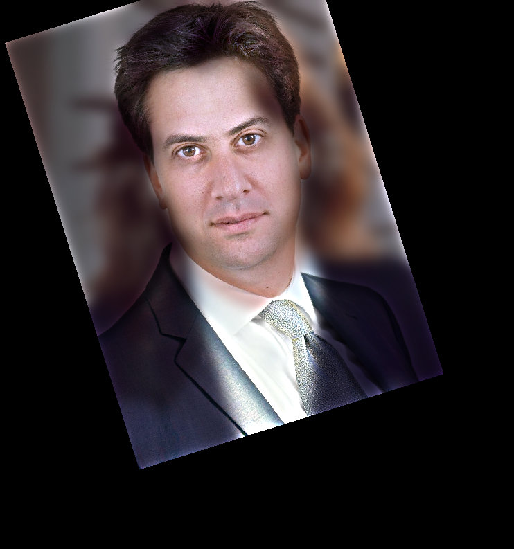
Which produces the following alignment:
3. Colour correcting the second image
If we tried to overlay facial features at this point, we’d soon see we have a problem:
The issue is that differences in skin-tone and lighting between the two images is causing a discontinuity around the edges of the overlaid region. Let’s try to correct that:
Dlib implements the algorithm described in the paper One Millisecond Face Alignment with an Ensemble of Regression Trees, by Vahid Kazemi and Josephine Sullivan. The algorithm itself is very complex, but dlib’s interface for using it is incredibly simple:
 1 COLOUR_CORRECT_BLUR_FRAC = 0.6
 2 LEFT_EYE_POINTS = list(range(42, 48))
 3 RIGHT_EYE_POINTS = list(range(36, 42))
 4
 5 def correct_colours(im1, im2, landmarks1):
 6     blur_amount = COLOUR_CORRECT_BLUR_FRAC * numpy.linalg.norm(
 7                               numpy.mean(landmarks1[LEFT_EYE_POINTS], axis=0) -
 8                               numpy.mean(landmarks1[RIGHT_EYE_POINTS], axis=0))
 9     blur_amount = int(blur_amount)
10     if blur_amount % 2 == 0:
11         blur_amount += 1
12     im1_blur = cv2.GaussianBlur(im1, (blur_amount, blur_amount), 0)
13     im2_blur = cv2.GaussianBlur(im2, (blur_amount, blur_amount), 0)
14
15     # Avoid divide-by-zero errors.
16     im2_blur += 128 * (im2_blur <= 1.0)
17
18     return (im2.astype(numpy.float64) * im1_blur.astype(numpy.float64) /
19                                                 im2_blur.astype(numpy.float64))
And the result:
This function attempts to change the colouring of im2 to match that of im1. It does this by dividing im2 by a gaussian blur of im2, and then multiplying by a gaussian blur of im1. The idea here is that of a RGB scaling colour-correction, but instead of a constant scale factor across all of the image, each pixel has its own localised scale factor.
With this approach differences in lighting between the two images can be accounted for, to some degree. For example, if image 1 is lit from one side but image 2 has uniform lighting then the colour corrected image 2 will appear darker on the unlit side aswell.
That said, this is a fairly crude solution to the problem and an appropriate size gaussian kernel is key. Too small and facial features from the first image will show up in the second. Too large and kernel strays outside of the face area for pixels being overlaid, and discolouration occurs. Here a kernel of 0.6 * the pupillary distance is used.
4. Blending features from the second image onto the first
A mask is used to select which parts of image 2 and which parts of image 1 should be shown in the final image:
Regions with value 1 (shown white here) correspond with areas where image 2 should show, and regions with colour 0 (shown black here) correspond with areas where image 1 should show. Value in between 0 and 1 correspond with a mixture of image 1 and image2.
Here’s the code to generate the above:
 1 LEFT_EYE_POINTS = list(range(42, 48))
 2 RIGHT_EYE_POINTS = list(range(36, 42))
 3 LEFT_BROW_POINTS = list(range(22, 27))
 4 RIGHT_BROW_POINTS = list(range(17, 22))
 5 NOSE_POINTS = list(range(27, 35))
 6 MOUTH_POINTS = list(range(48, 61))
 7 OVERLAY_POINTS = [
 8     LEFT_EYE_POINTS + RIGHT_EYE_POINTS + LEFT_BROW_POINTS + RIGHT_BROW_POINTS,
 9     NOSE_POINTS + MOUTH_POINTS,
10 ]
11 FEATHER_AMOUNT = 11
12
13 def draw_convex_hull(im, points, color):
14     points = cv2.convexHull(points)
15     cv2.fillConvexPoly(im, points, color=color)
16
17 def get_face_mask(im, landmarks):
18     im = numpy.zeros(im.shape[:2], dtype=numpy.float64)
19
20     for group in OVERLAY_POINTS:
21         draw_convex_hull(im,
22                          landmarks[group],
23                          color=1)
24
25     im = numpy.array([im, im, im]).transpose((1, 2, 0))
26
27     im = (cv2.GaussianBlur(im, (FEATHER_AMOUNT, FEATHER_AMOUNT), 0) > 0) * 1.0
28     im = cv2.GaussianBlur(im, (FEATHER_AMOUNT, FEATHER_AMOUNT), 0)
29
30     return im
31
32 mask = get_face_mask(im2, landmarks2)
33 warped_mask = warp_im(mask, M, im1.shape)
34 combined_mask = numpy.max([get_face_mask(im1, landmarks1), warped_mask],
35                           axis=0)