单细胞分析实录(6): 去除批次效应/整合数据

上一篇已经讲解了Seurat标准流程，推文的最后，注意到了不同样本之间的表达数据是存在批次效应的，就像下图这样，有些是可以聚到一起的亚群，却出现了不同样本分开/偏移的情况，比如第3群，这种就是批次效应：

接下来我会介绍Seurat v3的标准整合流程、Seurat结合Harmony 的整合流程，仍然使用上一个数据集

1. Seurat v3的标准整合流程

对于不同样本先分别运行Seurat的标准流程到找Variable基因这一步

library(Seurat)
library(tidyverse)
### testA ----
testA.seu=CreateSeuratObject(counts = testA)
testA.seu <- NormalizeData(testA.seu, normalization.method = "LogNormalize", scale.factor = 10000)
testA.seu <- FindVariableFeatures(testA.seu, selection.method = "vst", nfeatures = 2000)
### testB ----
testB.seu=CreateSeuratObject(counts = testB)
testB.seu <- NormalizeData(testB.seu, normalization.method = "LogNormalize", scale.factor = 10000)
testB.seu <- FindVariableFeatures(testB.seu, selection.method = "vst", nfeatures = 2000)

然后就是主要的整合步骤，object.list参数是由多个Seurat对象构成的列表，如下：

### Integration ----
testAB.anchors <- FindIntegrationAnchors(object.list = list(testA.seu,testB.seu), dims = 1:20)
testAB.integrated <- IntegrateData(anchorset = testAB.anchors, dims = 1:20)

需要注意的是：上面的整合步骤相对于harmony整合方法，对于较大的数据集（几万个细胞），非常消耗内存和时间；当存在某一个Seurat对象细胞数很少（印象中200以下这样子），会报错，这时建议用第二种整合方法

这一步之后就多了一个整合后的assay（原先有一个RNA的assay），整合前后的数据分别存储在这两个assay中

> testAB.integrated
An object of class Seurat 
35538 features across 6746 samples within 2 assays 
Active assay: integrated (2000 features)
 1 other assay present: RNA
 
 > dim(testAB.integrated[["RNA"]]@counts)
[1] 33538  6746
> dim(testAB.integrated[["RNA"]]@data)
[1] 33538  6746

> dim(testAB.integrated[["integrated"]]@counts) #因为是从RNA这个assay的data矩阵开始整合的，所以这个矩阵为空
[1] 0 0
> dim(testAB.integrated[["integrated"]]@data)
[1] 2000 6746

后续仍然是标准流程，基于上面得到的整合data矩阵

DefaultAssay(testAB.integrated) <- "integrated"
# Run the standard workflow for visualization and clustering
testAB.integrated <- ScaleData(testAB.integrated, features = rownames(testAB.integrated))
testAB.integrated <- RunPCA(testAB.integrated, npcs = 50, verbose = FALSE)
testAB.integrated <- FindNeighbors(testAB.integrated, dims = 1:30)
testAB.integrated <- FindClusters(testAB.integrated, resolution = 0.5)
testAB.integrated <- RunUMAP(testAB.integrated, dims = 1:30)
testAB.integrated <- RunTSNE(testAB.integrated, dims = 1:30)

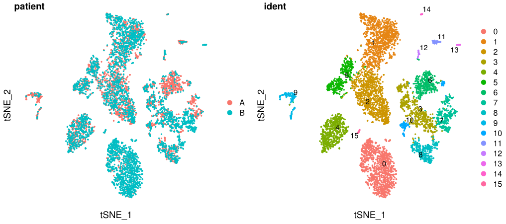
看一下去除批次效应之后的结果

library(cowplot)
testAB.integrated$patient=str_replace(testAB.integrated$orig.ident,"_.*$","")
p1 <- DimPlot(testAB.integrated, reduction = "tsne", group.by = "patient", pt.size=0.5)+theme(
  axis.line = element_blank(),
  axis.ticks = element_blank(),axis.text = element_blank()
)
p2 <- DimPlot(testAB.integrated, reduction = "tsne", group.by = "ident",   pt.size=0.5, label = TRUE,repel = TRUE)+theme(
  axis.line = element_blank(),
  axis.ticks = element_blank(),axis.text = element_blank()
)
fig_tsne <- plot_grid(p1, p2, labels = c('patient','ident'),align = "v",ncol = 2)
ggsave(filename = "tsne2.pdf", plot = fig_tsne, device = 'pdf', width = 27, height = 12, units = 'cm')

可以看到，不同样本的细胞基本都分散均匀了，结果还不错

2. Seurat结合Harmony的整合流程

这种整合方法很简单，而且占内存少，速度快

library(harmony)
testdf=cbind(testA,testB)
test.seu <- CreateSeuratObject(counts = testdf) %>%
  Seurat::NormalizeData() %>%
  FindVariableFeatures(selection.method = "vst", nfeatures = 2000) %>% 
  ScaleData()
test.seu <- RunPCA(test.seu, npcs = 50, verbose = FALSE)
test.seu@meta.data$patient=str_replace(test.seu$orig.ident,"_.*$","")

先运行Seurat标准流程到PCA这一步，然后就是Harmony整合，可以简单把这一步理解为一种新的降维

test.seu=test.seu %>% RunHarmony("patient", plot_convergence = TRUE)

> test.seu
An object of class Seurat 
33538 features across 6746 samples within 1 assay 
Active assay: RNA (33538 features)
 2 dimensional reductions calculated: pca, harmony

接着就是常规聚类降维，都是基于Harmony的Embeddings矩阵

test.seu <- test.seu %>% 
  RunUMAP(reduction = "harmony", dims = 1:30) %>% 
  FindNeighbors(reduction = "harmony", dims = 1:30) %>% 
  FindClusters(resolution = 0.5) %>% 
  identity()

test.seu <- test.seu %>% 
  RunTSNE(reduction = "harmony", dims = 1:30)

看看效果

p3 <- DimPlot(test.seu, reduction = "tsne", group.by = "patient", pt.size=0.5)+theme(
  axis.line = element_blank(),
  axis.ticks = element_blank(),axis.text = element_blank()
)
p4 <- DimPlot(test.seu, reduction = "tsne", group.by = "ident",   pt.size=0.5, label = TRUE,repel = TRUE)+theme(
  axis.line = element_blank(),
  axis.ticks = element_blank(),axis.text = element_blank()
)
fig_tsne <- plot_grid(p3, p4, labels = c('patient','ident'),align = "v",ncol = 2)
ggsave(filename = "tsne3.pdf", plot = fig_tsne, device = 'pdf', width = 27, height = 12, units = 'cm')

看起来也挺好的~

---

对于异质性很大的不同数据集，比如不同病人的肿瘤细胞，考虑到生物学差异已经远远大于批次效应，这时不应该再进行批次效应的去除，不然内在的生物学差异也会抹掉。尽管也在文献里面看到过对肿瘤细胞去批次的，但我始终觉得这样做是错的。不知道大家是怎么看的？

---

最后还有一个有用的小技巧，在降维之后，我们可以用DimPlot()函数把结果画在二维平面上，那这些坐标信息存储在哪儿呢？存储在Embeddings(test.seu,"pca")矩阵中，harmony/tsne/umap同理。有时候我们可以把坐标和meta@data的信息提取出来，用ggplot2画图，方便修改。

> Embeddings(test.seu,"tsne")[1:4,1:2]
                       tSNE_1    tSNE_2
A_AAACCCAAGGGTCACA  -6.774032 -25.08772
A_AAACCCAAGTATAACG  -5.294804  39.77550
A_AAACCCAGTCTCTCAC  30.600943  31.28015
A_AAACCCAGTGAGTCAG -32.432794 -14.62455

因水平有限，有错误的地方，欢迎批评指正！