在前一节最后,我们实现了一个将网络输出转换为检测预测的函数。现在我们已经有了一个检测器了,剩下的就是创建输入和输出的流程。
必要条件:
1.此系列教程的Part1到Part4。
2.Pytorch的基本知识,包括如何使用nn.Module,nn.Sequential,torch.nn.parameter类构建常规的结构
3.OpenCV的基础知识
EDIT: 如果你在2018年3月30日之前访问过这篇文章,我们将任意大小的图片调整为Darknet的输入大小的方法就是resize。然而在原始的实现中,调整图像的大小时,需要保持长宽比不变,并填充遗漏的部分。例如,如果我们将1900 x 1280的图像调整为416 x 415,那么调整后的图像应该是这样的。
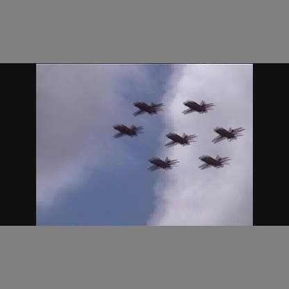
对于输入处理的差异导致早期实现的性能略低于原始实现。现在这篇文章已经进行了更新,遵循了原始实现中调整大小的方法。
在这一部分中,我们将构建检测器的输入和输出管道。这包括从磁盘读取图像,进行预测,使用预测结果在图像上绘制边界框,然后将它们保存到磁盘。我们还将介绍如何让检测器实时工作在一个摄像机或视频中。我们将介绍一些命令行标志,以允许对网络的各种超参数进行一些实验。那么让我们开始吧!
注意:这部分需要安装opencv3。
创建detector.py文件,在顶部添加必要的导入。
from __future__ import division
import time
import torch
import torch.nn as nn
from torch.autograd import Variable
import numpy as np
import cv2
from util import *
import argparse
import os
import os.path as osp
from darknet import Darknet
import pickle as pkl
import pandas as pd
import random
创建命令行参数:
因为detector.py是我们要执行来运行检测器的文件,所以最好有可以传递给它的命令行参数。我使用了python的ArgParse模块来实现这一点。
def arg_parse():
    """
    Parse arguements to the detect module

    """

    parser = argparse.ArgumentParser(description='YOLO v3 Detection Module')

    parser.add_argument("--images", dest = 'images', help =
                        "Image / Directory containing images to perform detection upon",
                        default = "imgs", type = str)
    parser.add_argument("--det", dest = 'det', help =
                        "Image / Directory to store detections to",
                        default = "det", type = str)
    parser.add_argument("--bs", dest = "bs", help = "Batch size", default = 1)
    parser.add_argument("--confidence", dest = "confidence", help = "Object Confidence to filter predictions", default = 0.5)
    parser.add_argument("--nms_thresh", dest = "nms_thresh", help = "NMS Threshhold", default = 0.4)
    parser.add_argument("--cfg", dest = 'cfgfile', help =
                        "Config file",
                        default = "cfg/yolov3.cfg", type = str)
    parser.add_argument("--weights", dest = 'weightsfile', help =
                        "weightsfile",
                        default = "yolov3.weights", type = str)
    parser.add_argument("--reso", dest = 'reso', help =
                        "Input resolution of the network. Increase to increase accuracy. Decrease to increase speed",
                        default = "416", type = str)

    return parser.parse_args()

args = arg_parse()
images = args.images
batch_size = int(args.bs)
confidence = float(args.confidence)
nms_thesh = float(args.nms_thresh)
start = 0
CUDA = torch.cuda.is_available()
其中,重要的标志是images(用于指定图像的输入图像或目录)、det(保存检测到的目录)、reso(输入图像的分辨率,可用于速度-精度权衡)、cfg(可更改的配置文件)和weightfile。
加载网络:
从这里下载coco.names文件,该文件包含COCO数据集中对象的名称。在检测器目录中创建文件夹数据。同样如果你在linux上工作,可以输入。
mkdir data
cd data
wget https://raw.githubusercontent.com/ayooshkathuria/YOLO_v3_tutorial_from_scratch/master/data/coco.name
然后,我们在程序中加载该文件。
num_classes = 80    #For COCO
classes = load_classes("data/coco.names")
load_classes是在util.py中定义的一个函数,它返回一个字典,该字典将每个类的索引映射到它的名称字符串。
def load_classes(namesfile):
    fp = open(namesfile, "r")
    names = fp.read().split("
")[:-1]
    return names
初始化网络并加载权重。
#Set up the neural network
print("Loading network.....")
model = Darknet(args.cfgfile)
model.load_weights(args.weightsfile)
print("Network successfully loaded")

model.net_info["height"] = args.reso
inp_dim = int(model.net_info["height"])
assert inp_dim % 32 == 0
assert inp_dim > 32

#If there's a GPU availible, put the model on GPU
if CUDA:
    model.cuda()

#Set the model in evaluation mode
model.eval()
读入输入图片:
从磁盘或目录中读取图像。将图像的路径存储在一个名为imlist的列表中。
read_dir = time.time()
#Detection phase
try:
    imlist = [osp.join(osp.realpath('.'), images, img) for img in os.listdir(images)]
except NotADirectoryError:
    imlist = []
    imlist.append(osp.join(osp.realpath('.'), images))
except FileNotFoundError:
    print ("No file or directory with the name {}".format(images))
    exit()
read_dir是一个用于度量时间的检查点。(大概就是判断每步花了多长时间)
如果保存检测的目录(由det标志定义)不存在,则创建它。
if not os.path.exists(args.det):
    os.makedirs(args.det)
我们将使用OpenCV来加载图像
load_batch = time.time()
loaded_ims = [cv2.imread(x) for x in imlist]
load_batch也是一个时间检查点
OpenCV以numpy数组的形式加载图像,以BGR作为颜色通道的顺序。PyTorch的图像输入格式为(批量x通道x高x宽),通道顺序为RGB。因此,我们在util.py中编写函数prep_image来将numpy数组转换为PyTorch的输入格式。
在编写这个函数之前,我们必须编写一个函数letterbox_image来调整图像的大小,保持长宽比一致,并用(128,128,128)填充余下区域
def letterbox_image(img, inp_dim):
    '''resize image with unchanged aspect ratio using padding'''
    img_w, img_h = img.shape[1], img.shape[0]
    w, h = inp_dim
    new_w = int(img_w * min(w/img_w, h/img_h))
    new_h = int(img_h * min(w/img_w, h/img_h))
    resized_image = cv2.resize(img, (new_w,new_h), interpolation = cv2.INTER_CUBIC)

    canvas = np.full((inp_dim[1], inp_dim[0], 3), 128)

    canvas[(h-new_h)//2:(h-new_h)//2 + new_h,(w-new_w)//2:(w-new_w)//2 + new_w,  :] = resized_image

    return canvas
现在我们编写一个函数,它获取OpenCV图像并将其转换为网络的输入。
def prep_image(img, inp_dim):
    """
    Prepare image for inputting to the neural network.

    Returns a Variable
    """

    img = cv2.resize(img, (inp_dim, inp_dim))
    img = img[:,:,::-1].transpose((2,0,1)).copy()
    img = torch.from_numpy(img).float().div(255.0).unsqueeze(0)
    return img
除了转换后的图像,我们还维护了原始图像列表和im_dim_list,后者包含原始图像的维度。
#PyTorch Variables for images
im_batches = list(map(prep_image, loaded_ims, [inp_dim for x in range(len(imlist))]))

#List containing dimensions of original images
im_dim_list = [(x.shape[1], x.shape[0]) for x in loaded_ims]
im_dim_list = torch.FloatTensor(im_dim_list).repeat(1,2)

if CUDA:
    im_dim_list = im_dim_list.cuda()
创建批:
leftover = 0
if (len(im_dim_list) % batch_size):
   leftover = 1

if batch_size != 1:
   num_batches = len(imlist) // batch_size + leftover
   im_batches = [torch.cat((im_batches[i*batch_size : min((i +  1)*batch_size,
                       len(im_batches))]))  for i in range(num_batches)]
检测循环体:
我们对批次进行迭代,生成预测并连接所有图像的预测张量(write_results函数的输出,维度为D*8)。
对于每个批,我们将检测所花费的时间定义为从接收输入到write_results函数产生输出之间所花费的时间。在write_prediction返回的输出中,其中一个属性是批中图像的索引。我们将其转换成在imlist中图像的索引,imlist列表包含所有图像的地址。
之后,我们打印每次检测所花费的时间以及在每张图像中检测到的对象。如果批的write_results函数的输出是int(0)就意味着没有检测,那么我们使用continue跳过rest循环。
write = 0
start_det_loop = time.time()
for i, batch in enumerate(im_batches):
    #load the image
    start = time.time()
    if CUDA:
        batch = batch.cuda()

    prediction = model(Variable(batch, volatile = True), CUDA)

    prediction = write_results(prediction, confidence, num_classes, nms_conf = nms_thesh)

    end = time.time()

    if type(prediction) == int:

        for im_num, image in enumerate(imlist[i*batch_size: min((i +  1)*batch_size, len(imlist))]):
            im_id = i*batch_size + im_num
            print("{0:20s} predicted in {1:6.3f} seconds".format(image.split("/")[-1], (end - start)/batch_size))
            print("{0:20s} {1:s}".format("Objects Detected:", ""))
            print("----------------------------------------------------------")
        continue

    prediction[:,0] += i*batch_size    #transform the atribute from index in batch to index in imlist

    if not write:                      #If we have't initialised output
        output = prediction
        write = 1
    else:
        output = torch.cat((output,prediction))

    for im_num, image in enumerate(imlist[i*batch_size: min((i +  1)*batch_size, len(imlist))]):
        im_id = i*batch_size + im_num
        objs = [classes[int(x[-1])] for x in output if int(x[0]) == im_id]
        print("{0:20s} predicted in {1:6.3f} seconds".format(image.split("/")[-1], (end - start)/batch_size))
        print("{0:20s} {1:s}".format("Objects Detected:", " ".join(objs)))
        print("----------------------------------------------------------")

    if CUDA:
        torch.cuda.synchronize()
torch.cuda.synchronize确保CUDA内核与CPU同步。否则CUDA内核会在GPU作业排队之后,甚至在GPU作业完成之前(异步调用)就将控制权返回给CPU。如果end = time() 在GPU作业实际结束之前打印出来,可能会导致错误的时间。
现在,我们已经在tensor输出中检测到了所有的图像。让我们在图像上绘制边界框吧!
在图像上绘制边界框:
我们使用try-catch块来检查是否进行了一次检测。如果没有则退出程序。
try:
    output
except NameError:
    print ("No detections were made")
    exit()
在绘制边界框之前,输出tensor中包含的预测符合网络的输入大小而不是图像的原始大小。因此,在绘制边界框之前,让我们将每个边界框的角属性转换为图像的原始维度。
在绘制边界框之前,输出tensor中包含的预测是对填充图像的预测,而不是对原始图像的预测。仅仅将它们重新缩放到输入图像的维数在这里是行不通的。首先,我们需要将边界框的坐标转换到相对于包含原始图像的填充图像上的边界。
im_dim_list = torch.index_select(im_dim_list, 0, output[:,0].long())

scaling_factor = torch.min(inp_dim/im_dim_list,1)[0].view(-1,1)


output[:,[1,3]] -= (inp_dim - scaling_factor*im_dim_list[:,0].view(-1,1))/2
output[:,[2,4]] -= (inp_dim - scaling_factor*im_dim_list[:,1].view(-1,1))/2
现在,我们的坐标匹配填充区域上图像部分的尺寸。然而,在函数letterbox_image中,我们通过缩放因子调整了图像的两个维度的大小(请记住,两个维度都用一个公共因子来划分,以保持长宽比)。现在,我们撤消这个重新缩放,以获得原始图像上的边框的坐标。
output[:,1:5] /= scaling_factor
因为有些边界框的可能超出了图像边缘,我们要将其限制在图片范围内。
for i in range(output.shape[0]):
    output[i, [1,3]] = torch.clamp(output[i, [1,3]], 0.0, im_dim_list[i,0])
    output[i, [2,4]] = torch.clamp(output[i, [2,4]], 0.0, im_dim_list[i,1])
如果图像中有很多边界框,用一种颜色绘制它们可能不太好。将此文件下载到检测器文件夹,这是一个pickle文件,其中包含许多颜色可供随机选择。
class_load = time.time()
colors = pkl.load(open("pallete", "rb"))
现在我们来写绘制边界框的函数。(x中的信息是图像索引、4个角坐标、目标置信度得分、最大置信类得分、该类的索引)
draw = time.time()

def write(x, results, color):
    c1 = tuple(x[1:3].int())
    c2 = tuple(x[3:5].int())
    img = results[int(x[0])]
    cls = int(x[-1])
    label = "{0}".format(classes[cls])
    cv2.rectangle(img, c1, c2,color, 1)
    t_size = cv2.getTextSize(label, cv2.FONT_HERSHEY_PLAIN, 1 , 1)[0]
    c2 = c1[0] + t_size[0] + 3, c1[1] + t_size[1] + 4
    cv2.rectangle(img, c1, c2,color, -1)
    cv2.putText(img, label, (c1[0], c1[1] + t_size[1] + 4), cv2.FONT_HERSHEY_PLAIN, 1, [225,255,255], 1);
    return img
上面的函数从colors中随机选择一个颜色来绘制矩形。它还在包围框的左上角创建一个填充矩形,并在填充矩形中写入检测到的对象的类。-1是cv2.rectangle函数用于创建填充矩形的参数。
我们的write函数是局部定义的以便它可以访问颜色列表。我们也可以用颜色作为参数,但是那样我们就只能用一种颜色。
完成这个函数定义后,现在让我们在图像上绘制边界框。
list(map(lambda x: write(x, loaded_ims), output))
上面的代码片段修改了loaded_ims中的图像。
在图像名称前面加上前缀“det_”然后保存每个图像。我们创建一个地址列表,并将检测图像保存到其中。
det_names = pd.Series(imlist).apply(lambda x: "{}/det_{}".format(args.det,x.split("/")[-1]))
最后,用det_names将检测到的图像写入地址。
list(map(cv2.imwrite, det_names, loaded_ims))
end = time.time()
打印时间日志:
在检测器的最后,我们将打印一个日志,其中包含执行代码的哪一部分花费了多长时间。这对我们比较不同的超参数如何影响检测器的速度时很重要。可以在命令行上执行脚本检测.py时设置超参数,如批大小、对象置信度和NMS阈值(分别通过bs、confidence和nms_thresh这些标志传递)。
print("SUMMARY")
print("----------------------------------------------------------")
print("{:25s}: {}".format("Task", "Time Taken (in seconds)"))
print()
print("{:25s}: {:2.3f}".format("Reading addresses", load_batch - read_dir))
print("{:25s}: {:2.3f}".format("Loading batch", start_det_loop - load_batch))
print("{:25s}: {:2.3f}".format("Detection (" + str(len(imlist)) +  " images)", output_recast - start_det_loop))
print("{:25s}: {:2.3f}".format("Output Processing", class_load - output_recast))
print("{:25s}: {:2.3f}".format("Drawing Boxes", end - draw))
print("{:25s}: {:2.3f}".format("Average time_per_img", (end - load_batch)/len(imlist)))
print("----------------------------------------------------------")


torch.cuda.empty_cache()
测试目标检测器:
在终端输入:
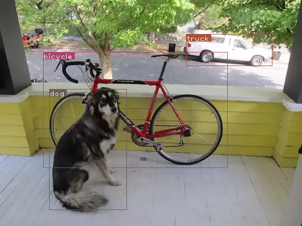
python detect.py --images dog-cycle-car.png --det det
产生输出:
Loading network.....
Network successfully loaded
dog-cycle-car.png    predicted in  2.456 seconds
Objects Detected:    bicycle truck dog
----------------------------------------------------------
SUMMARY
----------------------------------------------------------
Task                     : Time Taken (in seconds)

Reading addresses        : 0.002
Loading batch            : 0.120
Detection (1 images)     : 2.457
Output Processing        : 0.002
Drawing Boxes            : 0.076
Average time_per_img     : 2.657
将名为det_dog-cycle-car.png的图像保存在det目录中。
在视频/摄像机上运行检测器:
在视频或网络摄像头上运行检测器,代码几乎保持不变,只是我们不需要遍历批次,而是遍历视频的帧。
在github存储库中的video.py文件中可以找到在视频上运行检测器的代码。除了一些更改之外,代码与detector .py非常相似。
首先,在OpenCV中打开视频/摄像机流
videofile = "video.avi" #or path to the video file.

cap = cv2.VideoCapture(videofile)

#cap = cv2.VideoCapture(0)  for webcam

assert cap.isOpened(), 'Cannot capture source'

frames = 0
我们在帧上迭代的方式与在图像上迭代的方式相似。
许多地方都简化了很多代码,因为每次只需要处理一个图像,不再需要处理批。我们使用一个元组来代替im_dim_list的张量,在write函数中进行了微小的更改。
每次迭代时我们使用一个变量frames。然后我们用这个数字除以从第一个帧开始的时间,打印视频的FPS。
现在我们不是使用cv2将检测图像写入磁盘,而是用cv2.imshow显示绘制了边界框的图像。如果用户按下Q按钮,代码就会中断循环视频就此结束。
frames = 0
start = time.time()

while cap.isOpened():
    ret, frame = cap.read()

    if ret:
        img = prep_image(frame, inp_dim)
#        cv2.imshow("a", frame)
        im_dim = frame.shape[1], frame.shape[0]
        im_dim = torch.FloatTensor(im_dim).repeat(1,2)

        if CUDA:
            im_dim = im_dim.cuda()
            img = img.cuda()

        output = model(Variable(img, volatile = True), CUDA)
        output = write_results(output, confidence, num_classes, nms_conf = nms_thesh)


        if type(output) == int:
            frames += 1
            print("FPS of the video is {:5.4f}".format( frames / (time.time() - start)))
            cv2.imshow("frame", frame)
            key = cv2.waitKey(1)
            if key & 0xFF == ord('q'):
                break
            continue
        output[:,1:5] = torch.clamp(output[:,1:5], 0.0, float(inp_dim))

        im_dim = im_dim.repeat(output.size(0), 1)/inp_dim
        output[:,1:5] *= im_dim

        classes = load_classes('data/coco.names')
        colors = pkl.load(open("pallete", "rb"))

        list(map(lambda x: write(x, frame), output))

        cv2.imshow("frame", frame)
        key = cv2.waitKey(1)
        if key & 0xFF == ord('q'):
            break
        frames += 1
        print(time.time() - start)
        print("FPS of the video is {:5.2f}".format( frames / (time.time() - start)))
    else:
        break
结论:
在本系列教程中,我们从零开始实现了一个目标检测器,并为达到这个目标而欢呼。我认为能够写出高效的代码是深度学习实践者被低估的技能之一。无论你的想法多么具有革命性,除非你能对它进行测试,否则它毫无用处,为此你需要有很强的编程技能。
我还意识到,在深度学习中学习任何topic的最佳方法都是实现代码。当你在阅读一篇文章的时候一些细微之处你可能会错过,编程会迫使你注意topic的每个细微之处。我希望本系列教程能够作为一个练习,锻炼你作为一个深度学习实践者的技能。