Week2 Programming Assignment: Linear Regression

这是我Andrew NG的Week2的第一次编程作业，这其中有一些我所学到的东西，以博客的形式记录，随笔。

收获：

• 矩阵运算可以替代循环。

内容包括

1. univariate下
   • univariate任务下一个demo：
   • 数据集绘制为图像
   • 损失函数计算
   • 梯度下降
2. multivariate任务下
   • 损失函数代码，梯度下降代码与上述一致（实用矩阵和向量化，从一开始就兼容了多变量的情况）
   • normal equation替代梯度下降计算参数　　
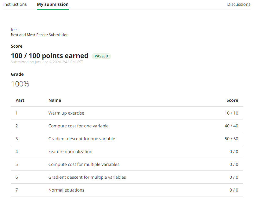
3. 提交结果
4. 分数

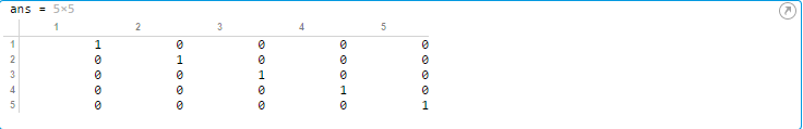
function A = warmUpExercise()
%WARMUPEXERCISE Example function in octave
%   A = WARMUPEXERCISE() is an example function that returns the 5x5 identity matrix

A = [];
% ============= YOUR CODE HERE ==============
% Instructions: Return the 5x5 identity matrix 
%               In octave, we return values by defining which variables
%               represent the return values (at the top of the file)
%               and then set them accordingly. 
A=eye(5);
% ===========================================
end

运行效果

function plotData(x, y)
%PLOTDATA Plots the data points x and y into a new figure 
%   PLOTDATA(x,y) plots the data points and gives the figure axes labels of
%   population and profit.

figure; % open a new figure window

% ====================== YOUR CODE HERE ======================
% Instructions: Plot the training data into a figure using the 
%               "figure" and "plot" commands. Set the axes labels using
%               the "xlabel" and "ylabel" commands. Assume the 
%               population and revenue data have been passed in
%               as the x and y arguments of this function.
%
% Hint: You can use the 'rx' option with plot to have the markers
%       appear as red crosses. Furthermore, you can make the
%       markers larger by using plot(..., 'rx', 'MarkerSize', 10);


plot(x, y, 'rx', 'MarkerSize', 10); % Plot the data
ylabel('Profit in $10,000s'); % Set the y?axis label
xlabel('Population of City in 10,000s'); % Set the x?axis label
% ============================================================

end

运行效果

function J = computeCost(X, y, theta)
%COMPUTECOST Compute cost for linear regression
%   J = COMPUTECOST(X, y, theta) computes the cost of using theta as the
%   parameter for linear regression to fit the data points in X and y

% Initialize some useful values
m = length(y); % number of training examples

% You need to return the following variables correctly 
J = 0;

% ====================== YOUR CODE HERE ======================
% Instructions: Compute the cost of a particular choice of theta
%               You should set J to the cost.
h_theta = X*theta;
sum_vector =ones(1,m);
J=sum_vector*((h_theta-y).^2)/(2*m);



% =========================================================================

end

运行效果

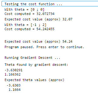
function [theta, J_history] = gradientDescent(X, y, theta, alpha, num_iters)
%GRADIENTDESCENT Performs gradient descent to learn theta
%   theta = GRADIENTDESCENT(X, y, theta, alpha, num_iters) updates theta by 
%   taking num_iters gradient steps with learning rate alpha

% Initialize some useful values
m = length(y); % number of training examples
J_history = zeros(num_iters, 1);

for iter = 1:num_iters

    % ====================== YOUR CODE HERE ======================
    % Instructions: Perform a single gradient step on the parameter vector
    %               theta. 
    %
    % Hint: While debugging, it can be useful to print out the values
    %       of the cost function (computeCost) and gradient here.
    %
    h_theta = X*theta;
    errors_vector=h_theta-y;
    theta_change = (X'*errors_vector)*alpha/(m);
    theta=theta-theta_change;
    % ============================================================
    
    % Save the cost J in every iteration    
    J_history(iter) = computeCost(X, y, theta);

end

end

运行效果

 

 进行数据拟合并预测

 损失函数三维立体图像

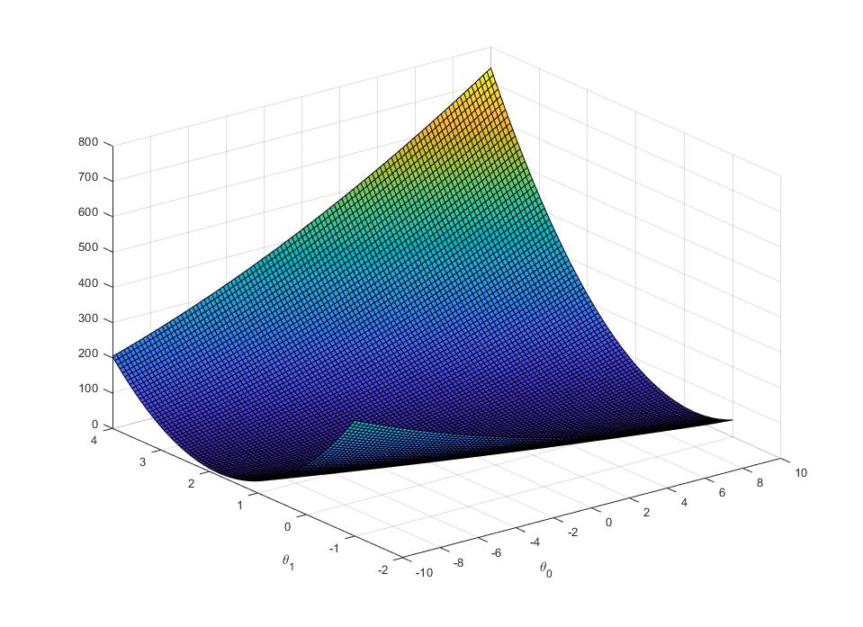
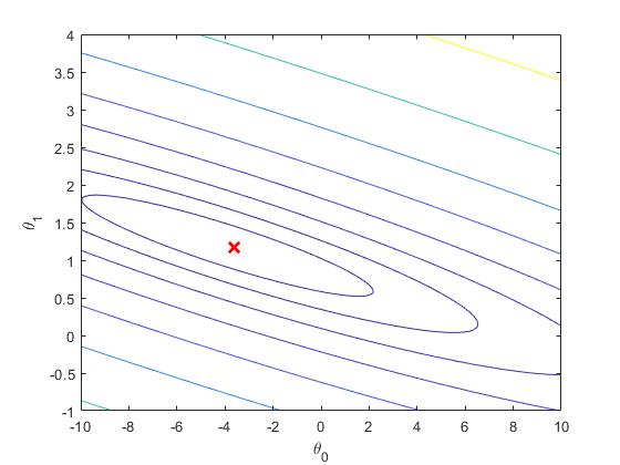
等高线

function [theta] = normalEqn(X, y)
%NORMALEQN Computes the closed-form solution to linear regression 
%   NORMALEQN(X,y) computes the closed-form solution to linear 
%   regression using the normal equations.

theta = zeros(size(X, 2), 1);

% ====================== YOUR CODE HERE ======================
% Instructions: Complete the code to compute the closed form solution
%               to linear regression and put the result in theta.
%

% ---------------------- Sample Solution ----------------------


theta=pinv(X'*X)*X'*y;

% -------------------------------------------------------------


% ============================================================

end

computeCostMulti和gradientDescentMulti与上面univariate一致

最终结果

>> submit
== Submitting solutions | Linear Regression with Multiple Variables...
Use token from last successful submission (yuhang.tao.email@gmail.com)? (Y/n): Y
== 
==                                   Part Name |     Score | Feedback
==                                   --------- |     ----- | --------
==                            Warm-up Exercise |  10 /  10 | Nice work!
==           Computing Cost (for One Variable) |  40 /  40 | Nice work!
==         Gradient Descent (for One Variable) |  50 /  50 | Nice work!
==                       Feature Normalization |   0 /   0 | Nice work!
==     Computing Cost (for Multiple Variables) |   0 /   0 | Nice work!
==   Gradient Descent (for Multiple Variables) |   0 /   0 | Nice work!
==                            Normal Equations |   0 /   0 | Nice work!
==                                   --------------------------------
==                                             | 100 / 100 | 
== 

Coursera上不对选做题加分