1.Tensorflow的模型到底是什么样的?
Tensorflow模型主要包含网络的设计(图)和训练好的各参数的值等。所以,Tensorflow模型有两个主要的文件:
a) Meta graph:
这是一个协议缓冲区(protocol buffer),它完整地保存了Tensorflow图;即所有的变量、操作、集合等。此文件以 .meta 为拓展名。
b) Checkpoint 文件:
这是一个二进制文件,包含weights、biases、gradients 和其他所有变量的值。此文件以 .ckpt 为扩展名. 但是,从Tensorflow 0.11版本之后做出了一些改变。现在,不再是单一的 .ckpt 文件,而是两个文件(.data和.index).data文件包含了我们的训练变量,稍后再说。
另外,Tensorflow还有一个名为 checkpoint 的文件,仅用于保存最新checkpoint文件保存的记录。

2. 保存一个Tensorflow模型:
比方说你正在训练一个卷积神经网络用于图像分类,你会关注于loss值和accuracy. 一旦你看到网络converged, 你就可以手工停止训练或设置固定的训练迭代次数。训练完成之后,我们想把所有变量值和网络图保存到文件中方便以后使用。所以,为了保存Tensorflow中的图和所有参数的值,我们创建一个tf.train.Saver()类的实例。
saver = tf.train.Saver()
别忘了Tensorflow变量仅存在于session内,所以你必须在session内进行保存,可通过调用创建的saver对象的sava方法实现。
saver.save(sess, path+"model_conv/my-model", global_step=epoch)
其中,sess是session对象,path+"model_conv/my-model"是你对自己模型的路径+命名,global_step表示迭代多少次就保存模型(比如每迭代1000次后保存模型:global_step=1000);如果你想保存最近的4个模型并且每训练两个小时保存一次,可以使用 max_to_keep=4 和 keep_checkpoint_every_n_hours=2
如果我们没有在tf.train.Saver()中指定任何参数,它会保存所有变量。如果我们不想保存全部变量而只是想保存一部分的话,我们可以指定想保存的variables/collections.在创建tf.train.Saver实例时,我们将它传递给我们想要保存的变量的列表或字典。看一个例子:
path = '/data/User/zcc/'
import tensorflow as tf

v1 = tf.Variable(tf.constant(1.0, shape=[1]), name="v1")
v2 = tf.Variable(tf.constant(2.0, shape=[1]), name="v2")
result = v1 + v2
saver = tf.train.Saver([v1,v2])
with tf.Session() as sess:
    sess.run(tf.global_variables_initializer())
    saver.save(sess, path+"Model_new/model.ckpt")
3.实战详解(简单的卷积神经网络)
下面定义了一个简单的卷积神经网络:有两个卷积层、两个池化层和两个全连接层。并且加载的数据是无意义的数据,模拟的是10张32x32的RGB图像,共4个类别0、1、2、3。这里主要是为了学习模型的保存和调用,对于数据怎样得来和准确率不用在意。
import tensorflow as tf
import numpy as np
import os
# 自定义要加载的训练集
def load_data(resultpath):

    datapath = os.path.join(resultpath, "data10_4.npz")
    # 如果有已经存在的数据,则加载
    if os.path.exists(datapath):
        data = np.load(datapath)
        # 注意提取数值的方法
        X, Y = data["X"], data["Y"]
    else:
        # 加载的数据是无意义的数据,模拟的是10张32x32的RGB图像,共4个类别:0、1、2、3
        # 将30720个数字化成10*32*32*32*3的张量
        X = np.array(np.arange(30720)).reshape(10, 32, 32, 3)
        Y = [0, 0, 1, 1, 2, 2, 3, 3, 2, 0]
        X = X.astype('float32')
        Y = np.array(Y)
        # 把数据保存成dataset.npz的格式
        np.savez(datapath, X=X, Y=Y)
        print('Saved dataset to dataset.npz')
    # 一种很好用的打印输出显示方式
    print('X_shape:{}
Y_shape:{}'.format(X.shape, Y.shape))
    return X, Y
# 搭建卷积网络:有两个卷积层、两个池化层和两个全连接层。
def define_model(x):
    x_image = tf.reshape(x, [-1, 32, 32, 3])
    print ('x_image.shape:',x_image.shape)
    def weight_variable(shape):
        initial = tf.truncated_normal(shape, stddev=0.1)
        return tf.Variable(initial, name="w")
    def bias_variable(shape):
        initial = tf.constant(0.1, shape=shape)
        return tf.Variable(initial, name="b")
    def conv3d(x, W):
        return tf.nn.conv2d(x, W, strides=[1, 1, 1, 1], padding='SAME')
    def max_pool_2d(x):
        return tf.nn.max_pool(x, ksize=[1, 3, 3, 1], strides=[1, 3, 3, 1], padding='SAME')

    with tf.variable_scope("conv1"):  # [-1,32,32,3]
        weights = weight_variable([3, 3, 3, 32])
        biases = bias_variable([32])
        conv1 = tf.nn.relu(conv3d(x_image, weights) + biases)
        pool1 = max_pool_2d(conv1)  # [-1,11,11,32]
    with tf.variable_scope("conv2"):
        weights = weight_variable([3, 3, 32, 64])
        biases = bias_variable([64])
        conv2 = tf.nn.relu(conv3d(pool1, weights) + biases)
        pool2 = max_pool_2d(conv2) # [-1,4,4,64]

    with tf.variable_scope("fc1"):
        weights = weight_variable([4 * 4 * 64, 128]) # [-1,1024]
        biases = bias_variable([128])
        fc1_flat = tf.reshape(pool2, [-1, 4 * 4 * 64])
        fc1 = tf.nn.relu(tf.matmul(fc1_flat, weights) + biases)
        fc1_drop = tf.nn.dropout(fc1, 0.5) # [-1,128]

    with tf.variable_scope("fc2"):
        weights = weight_variable([128, 4])
        biases = bias_variable([4])
        fc2 = tf.matmul(fc1_drop, weights) + biases # [-1,4]

    return fc2
path = '/data/User/zcc/'
# 训练模型
def train_model():

    # 训练数据的占位符
    x = tf.placeholder(tf.float32, shape=[None, 32, 32, 3], name="x")
    y_ = tf.placeholder('int64', shape=[None], name="y_")
    # 学习率
    initial_learning_rate = 0.001
    # 定义网络结构,前向传播,得到预测输出
    y_fc2 = define_model(x)
    # 定义训练集的one-hot标签
    y_label = tf.one_hot(y_, 4, name="y_labels")
    # 定义损失函数
    loss_temp = tf.losses.softmax_cross_entropy(onehot_labels=y_label, logits=y_fc2)
    cross_entropy_loss = tf.reduce_mean(loss_temp)

    # 训练时的优化器
    train_step = tf.train.AdamOptimizer(learning_rate=initial_learning_rate, beta1=0.9, beta2=0.999,
                                        epsilon=1e-08).minimize(cross_entropy_loss)

    # 一样返回True,否则返回False
    correct_prediction = tf.equal(tf.argmax(y_fc2, 1), tf.argmax(y_label, 1))
    # 将correct_prediction,转换成指定tf.float32类型
    accuracy = tf.reduce_mean(tf.cast(correct_prediction, tf.float32))

    # 保存模型,这里做多保存4个模型
    saver = tf.train.Saver(max_to_keep=4)
    # 把预测值加入predict集合
    tf.add_to_collection("predict", y_fc2)
    tf.add_to_collection("acc", accuracy )

    # 定义会话
    with tf.Session() as sess:
        # 所有变量初始化
        sess.run(tf.global_variables_initializer())
        print ("------------------------------------------------------")
        # 加载训练数据,这里的训练数据是构造的,旨在保存/加载模型的学习
        X, Y = load_data(path+"model_conv/") # 这里需要提前新建一个文件夹
        X = np.multiply(X, 1.0 / 255.0)

        for epoch in range(200):

            if epoch % 10 == 0:
                print ("------------------------------------------------------")
                train_accuracy = accuracy.eval(feed_dict={x: X, y_: Y})
                train_loss = cross_entropy_loss.eval(feed_dict={x: X, y_: Y})
                print ("after epoch %d, the loss is %6f" % (epoch, train_loss))
                # 这里的正确率是以整体的训练样本为训练样例的
                print ("after epoch %d, the acc is %6f" % (epoch, train_accuracy))
                saver.save(sess, path+"model_conv/my-model", global_step=epoch)
                print ("save the model")
            train_step.run(feed_dict={x: X, y_: Y})
        print ("------------------------------------------------------")
# 训练模型
train_model()
训练结果:
('x_image.shape:', TensorShape([Dimension(None), Dimension(32), Dimension(32), Dimension(3)]))
------------------------------------------------------
Saved dataset to dataset.npz
X_shape:(10, 32, 32, 3)
Y_shape:(10,)
------------------------------------------------------
after epoch 0, the loss is 91.338860
after epoch 0, the acc is 0.200000
save the model
------------------------------------------------------
after epoch 10, the loss is 19.594559
after epoch 10, the acc is 0.200000
save the model
------------------------------------------------------
after epoch 20, the loss is 5.181785
after epoch 20, the acc is 0.300000
save the model
------------------------------------------------------
after epoch 30, the loss is 2.592906
after epoch 30, the acc is 0.400000
save the model
------------------------------------------------------
after epoch 40, the loss is 1.611863
after epoch 40, the acc is 0.300000
save the model
------------------------------------------------------
after epoch 50, the loss is 1.317069
after epoch 50, the acc is 0.300000
save the model
------------------------------------------------------
after epoch 60, the loss is 1.313013
after epoch 60, the acc is 0.400000
save the model
------------------------------------------------------
after epoch 70, the loss is 1.268448
after epoch 70, the acc is 0.200000
save the model
------------------------------------------------------
after epoch 80, the loss is 1.323944
after epoch 80, the acc is 0.300000
save the model
------------------------------------------------------
after epoch 90, the loss is 1.276046
after epoch 90, the acc is 0.300000
save the model
------------------------------------------------------
after epoch 100, the loss is 1.284416
after epoch 100, the acc is 0.300000
save the model
------------------------------------------------------
after epoch 110, the loss is 1.254741
after epoch 110, the acc is 0.300000
save the model
------------------------------------------------------
after epoch 120, the loss is 1.354204
after epoch 120, the acc is 0.300000
save the model
------------------------------------------------------
after epoch 130, the loss is 1.253812
after epoch 130, the acc is 0.300000
save the model
------------------------------------------------------
after epoch 140, the loss is 1.169439
after epoch 140, the acc is 0.200000
save the model
------------------------------------------------------
after epoch 150, the loss is 1.263069
after epoch 150, the acc is 0.500000
save the model
------------------------------------------------------
after epoch 160, the loss is 1.257510
after epoch 160, the acc is 0.400000
save the model
------------------------------------------------------
after epoch 170, the loss is 1.223609
after epoch 170, the acc is 0.500000
save the model
------------------------------------------------------
after epoch 180, the loss is 1.214603
after epoch 180, the acc is 0.500000
save the model
------------------------------------------------------
after epoch 190, the loss is 1.237759
after epoch 190, the acc is 0.500000
save the model
------------------------------------------------------
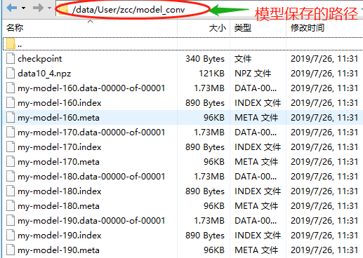
保存模型的文件夹内容如下:
# 利用保存的模型预测新的值,并计算准确值acc
path = '/data/User/zcc/'
def load_model():
    # 测试数据构造:模拟2张32x32的RGB图
    X = np.array(np.arange(6144, 12288)).reshape(2, 32, 32, 3)   #2:张,32*32:图片大小,3:RGB
    Y = [3, 1]
    Y = np.array(Y)
    X = X.astype('float32')
    X = np.multiply(X, 1.0 / 255.0)

    with tf.Session() as sess:
        # 加载元图和权重
        saver = tf.train.import_meta_graph(path+'model_conv/my-model-190.meta')
        saver.restore(sess, tf.train.latest_checkpoint(path+"model_conv/"))

        # 获取权重
        graph = tf.get_default_graph()  #获取当前默认计算图
        fc2_w = graph.get_tensor_by_name("fc2/w:0") #get_tensor_by_name后面传入的参数,如果没有重复,需要在后面加上“:0”
        fc2_b = graph.get_tensor_by_name("fc2/b:0")
        print ("------------------------------------------------------")
        #print ('fc2_w:',sess.run(fc2_w))可以打印查看,这里因为数据太多了,显示太占地方了,就不打印了
        print ("#######################################")
        print ('fc2_b:',sess.run(fc2_b))
        print ("------------------------------------------------------")

        # 预测输出
        feed_dict = {"x:0":X, "y_:0":Y}
        y = graph.get_tensor_by_name("y_labels:0")
        yy = sess.run(y, feed_dict) #将Y转为one-hot类型
        print ('yy:',yy)
        print ("the answer is: ", sess.run(tf.argmax(yy, 1)))
        print ("------------------------------------------------------")

        pred_y = tf.get_collection("predict")  #拿到原来模型中的"predict",也就是原来模型中计算得到结果y_fc2
        print('我用加载的模型来预测新输入的值了!')
        pred = sess.run(pred_y, feed_dict)[0] #利用原来计算y_fc2的方式计算新喂给网络的数据,即feed_dict = {"x:0":X, "y_:0":Y}
        print ('pred:',pred, '
')   #pred是新数据下得到的预测值
        pred = sess.run(tf.argmax(pred, 1))
        print ("the predict is: ", pred)
        print ("------------------------------------------------------")


        acc = tf.get_collection("acc")  #同样利用原模型中的计算图acc来计算新预测的准确值
        #acc = graph.get_operation_by_name("acc")
        acc = sess.run(acc, feed_dict) #acc是新数据下得到的准确值
        #print(acc.eval())
        print ("the accuracy is: ", acc)
        print ("------------------------------------------------------")
load_model()
运行结果:
------------------------------------------------------
#######################################
('fc2_b:', array([0.10513018, 0.07008364, 0.15466481, 0.06231203], dtype=float32))
------------------------------------------------------
('yy:', array([[0., 0., 0., 1.],
       [0., 1., 0., 0.]], dtype=float32))
('the answer is: ', array([3, 1]))
------------------------------------------------------
我用加载的模型来预测新输入的值了!
('pred:', array([[ 0.54676336, -0.07104626, -0.02205519, -0.24077414],
       [ 0.10513018,  0.07008364,  0.15466481,  0.06231203]],
      dtype=float32), '
')
('the predict is: ', array([0, 2]))
------------------------------------------------------
('the accuracy is: ', [0.0, 0.0])
------------------------------------------------------
4.模型微调fine-tuning
使用已经预训练好的模型,自己fine-tuning。首先获得pre-traing的graph结构
saver = tf.train.import_meta_graph(path+'my_test_model-1000.meta')
加载参数
saver.restore(sess,tf.train.latest_checkpoint(path))
准备feed_dict:新的训练数据或者测试数据。这样就可以使用同样的模型,训练或者测试不同的数据。
如果想在已有的网络结构上添加新的层,如前面卷积网络,获得fc2时,然后添加了一个全连接层和输出层。(这里的添加网络层没有进行测试)
# pre-train and fine-tuning
fc2 = graph.get_tensor_by_name("fc2/add:0")
fc2 = tf.stop_gradient(fc2)  # 将模型的一部分进行冻结
fc2_shape = fc2.get_shape().as_list()
# fine -tuning
new_nums = 6
weights = tf.Variable(tf.truncated_normal([fc2_shape[1], new_nums], stddev=0.1), name="w")
biases = tf.Variable(tf.constant(0.1, shape=[new_nums]), name="b")
conv2 = tf.matmul(fc2, weights) + biases
output2 = tf.nn.softmax(conv2)
参考博客: