目录:
一、face_recognition是什么
二、如何安装
三、原理
四、演示
五、手写简单的神经网络
一、face_recognition是什么
1. face_recognition是一个强大、简单、易上手的人脸识别开源项目,并且配备了完整的开发文档和应用案例。
2. 基于业内领先的C++开源库 dlib中的深度学习模型,用Labeled Faces in the Wild人脸数据集进行测试,有高达99.38%的准确率。
二、 如何安装
Linux下配置face_recognition
具体详情参考我的博客 https://www.cnblogs.com/UniqueColor/p/10992407.html
1、如linux下已有python2.7,但需要更新一下python 2.7至python2.x
sudo add-apt-repository ppa:fkrull/deadsnakes-python2.7
sudo apt-get update
sudo apt-get upgrade
2、部署步骤
安装Boost, Boost.Python
sudo apt-get install build-essential cmake
sudo apt-get install libgtk-3-dev
sudo apt-get install libboost-all-dev
Installation of Cmake:(it tooks a while to install ~1.5 min)
1 sudo wget  https://cmake.org/files/v3.9/cmake-3.9.0-rc5.tar.gz -O cmake.tar.gz
2 sudo tar -xvf cmake.tar.gz
3 cd cmake-3.9.0-rc5/
4 sudo chmod +x bootstrap
5 sudo ./bootstrap
6 sudo make
7 sudo make install

注:安装好cmake后,输入cmake -version查看cmake版本是否安装成功。
pip installation
$ wget https://bootstrap.pypa.io/get-pip.py
$ sudo python get-pip.py

注:安装完成后,终端输入pip -V查看pip版本是否安装成功。
注:如果使用python3.x版本,最后一步命令python改为python3
通过手动编译dlib的方式进行安装dlib
git clone https://github.com/davisking/dlib.git  //Clone the code from github
cd dlib
mkdir build
cd build
cmake ..                          //以默认方式(SSE41指令)编译dlib
cmake --build .
cd ..
sudo python setup.py install

注:最后一步需要等待一些时间。如果使用python3.x版本,最后一步命令python改为python3
安装完成后,运行python,输入 import dlib 此时执行成功。
安装face_recognition
sudo pip install face_recognition
安装完成后,运行python,输入 import face_recognition 此时执行成功。
安装opencv-python
pip install -i https://pypi.tuna.tsinghua.edu.cn/simple opencv-python
测试:运行python,输入 import cv2 此时执行成功。
Mac下配置face_recognition
具体详情参考我的博客 https://www.cnblogs.com/UniqueColor/p/10992415.html
安装依赖库:
1、安装cmake (是一个跨平台的安装工具)
brew install cmake
2、安装boost、boost-python(C++的程序库)
brew install boost
brew install boost-python --with-python2.7
3、编译dlib
git clone https://github.com/davisking/dlib.git
cd dlib
mkdir build
cd build
cmake ..                          //以默认方式(SSE41指令)编译dlib
cmake --build .
cd ..
sudo python setup.py install
4. 安装人脸识别的python库
pip install face_recognition
5、安装opencv-python
pip install -i https://pypi.tuna.tsinghua.edu.cn/simple opencv-python
此时报错:
Cannot uninstall 'numpy'. It is a distutils installed project and thus we cannot accurate
解决方案:强行升级
pip install numpy --ignore-installed numpy
三、原理:
1. HOG
HOG是什么?
HOG即方向梯度直方图。特征是一种在计算机视觉和图像处理中用来进行物体检测的特征描述子。HOG特征通过计算和统计图像局部区域的梯度方向直方图来构成特征。
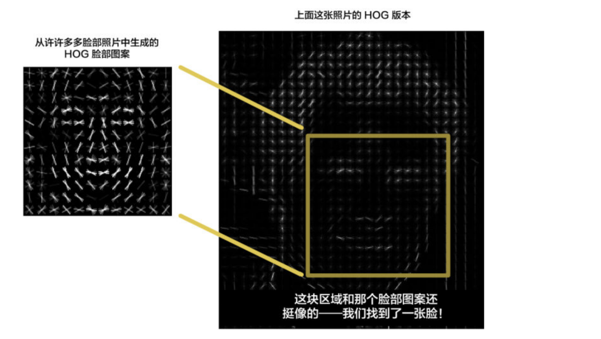
使用 HOG 算法给图片编码,以创建图片的简化版本。 使用这个简化的图像,找到其中看起来最像通用 HOG 面部编码的部分。
步骤:
1.1 将图像转换为黑白,为了降维,不用考虑色彩
1.2 查看图片中的每一个像素。 对于单个像素,同时要查看它周围的其他像素。目的是找出并比较当前像素与直接围绕它的像素的深度,形成箭头方向。通过对图片中的每一个像素重复这个过程,最终每个像素会被一个箭头取代。这些箭头被称为梯度(gradients),它们能显示出图像上从明亮到黑暗的流动过程。(使用梯度替代像素的原因是,同一个人在明暗不同的两张照片中具有不同的像素,但是如果只是分析梯度,明暗不同的两张照片也会得到相同的结果)。
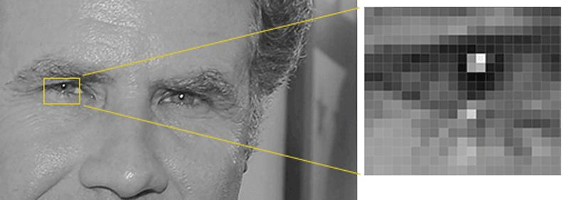
1.3 计算每一个像素未免太繁琐,所以将图像分割成一些 16×16 像素的小方块。在每个小方块中,我们将计算出每个主方向上有多少个梯度(有多少指向上,指向右上,指向右等)。然后我们将用指向性最强那个方向的箭头来代替原来的那个小方块。
具体文字算法步骤:
1、读入检测图片即输入的image
2、将图像灰度化(即将输入的彩色的图像的r,g,b值通过特定公式转换为灰度值)
3、采用Gamma校正法对输入图像进行颜色空间的标准化(归一化)
4、计算图像每个像素的梯度(包括大小和方向),捕获轮廓信息。如果我们直接分析像素,同一个人明暗不同的两张照片将具有完全不同的像素值。但是如果只考虑亮度变化方向(direction)的话,明暗图像将会有同样的结果
5、统计每个cell的梯度直方图(不同梯度的个数),形成每个cell的descriptor
6、将每几个cell(如上文提到的16*16)组成一个block,一个block内所有cell的特征串联起来得到该block的HOG特征descriptor
7、将image里所有block的HOG特征descriptor串联起来得到该image(检测目标)的HOG特征descriptor,得到最终分类的特征向量
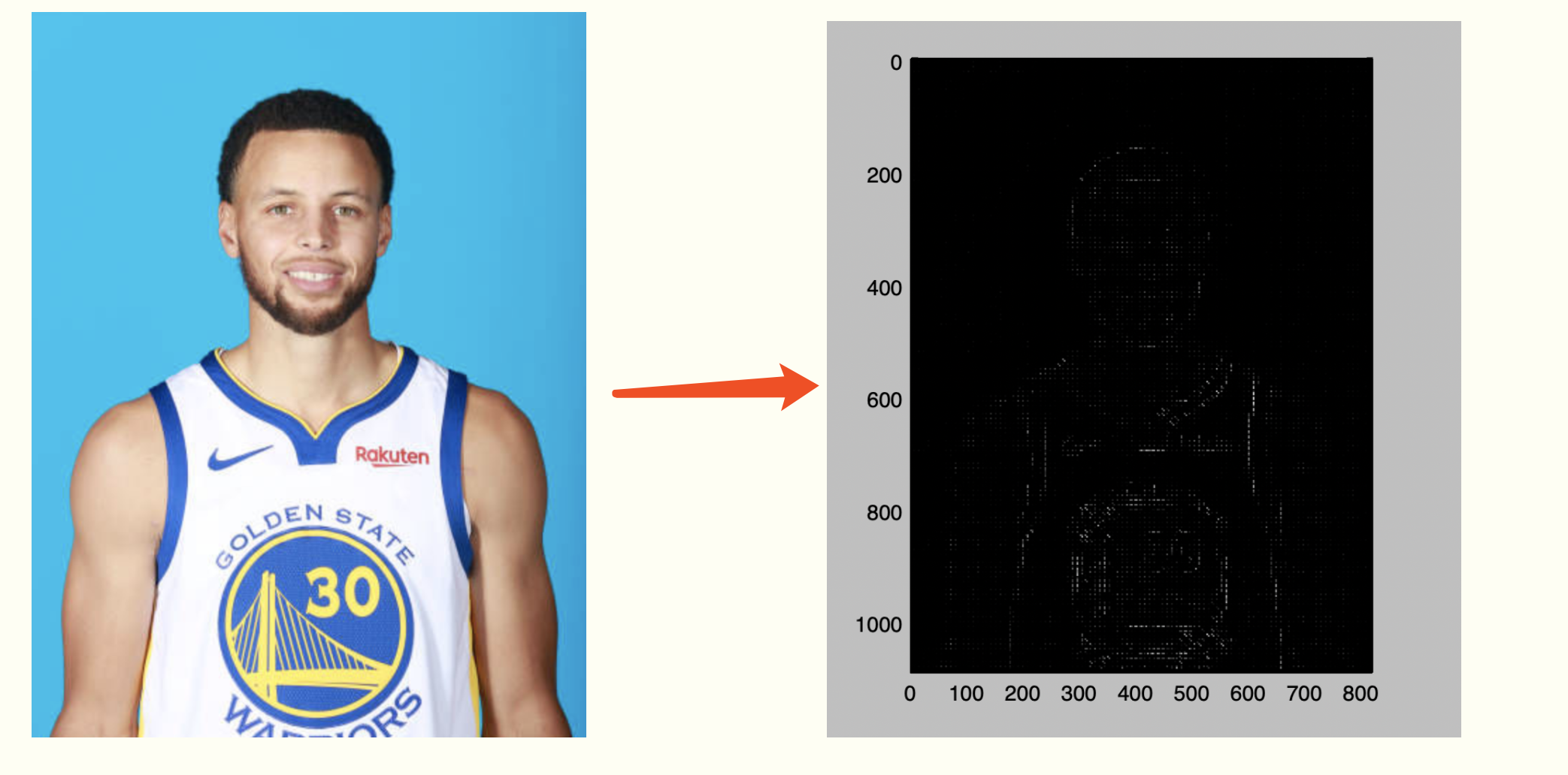
附上HOG实现代码:
  1 # coding=utf-8
  2 import cv2
  3 import numpy as np
  4 import math
  5 import matplotlib.pyplot as plt
  6
  7 # 1、读入检测图片即输入的image
  8 # 2、将图像灰度化(即将输入的彩色的图像的r,g,b值通过特定公式转换为灰度值)
  9 # 3、采用Gamma校正法对输入图像进行颜色空间的标准化(归一化)
 10 # 4、计算图像每个像素的梯度(包括大小和方向),捕获轮廓信息。如果我们直接分析像素,同一个人明暗不同的两张照片将具有完全不同的像素值。但是如果只考虑亮度变化方向(direction)的话,明暗图像将会有同样的结果
 11 # 5、统计每个cell的梯度直方图(不同梯度的个数),形成每个cell的descriptor
 12 # 6、将每几个cell(如上文提到的16*16)组成一个block,一个block内所有cell的特征串联起来得到该block的HOG特征descriptor
 13 # 7、将image里所有block的HOG特征descriptor串联起来得到该image(检测目标)的HOG特征descriptor,得到最终分类的特征向量
 14
 15 class Hog_descriptor():
 16     def __init__(self, img, cell_size=16, bin_size=8):
 17         # 数据处理
 18         self.img = img
 19         # 采用Gamma校正法对输入图像进行颜色空间的标准化(归一化),调节图像的对比度
 20         self.img = np.sqrt(img / np.max(img))
 21
 22         self.img = img * 255
 23         self.cell_size = cell_size
 24         self.bin_size = bin_size
 25         self.angle_unit = 360 / self.bin_size
 26
 27     def extract(self):
 28         height, width = self.img.shape
 29         # 1、计算每个像素的梯度
 30         gradient_magnitude, gradient_angle = self.global_gradient()
 31         gradient_magnitude = abs(gradient_magnitude)
 32
 33         # 2、开始为细胞单元构建梯度方向直方图
 34         cell_gradient_vector = np.zeros(
 35             (height / self.cell_size, width / self.cell_size, self.bin_size))  # 初始化8个直方图构成的向量组,即构成细胞元,前面两个参数表示每个直方图长和宽
 36         # 3、以直方图为单位 循环填充所有细胞元
 37         for i in range(cell_gradient_vector.shape[0]):
 38             for j in range(cell_gradient_vector.shape[1]):
 39                 cell_magnitude = gradient_magnitude[i * self.cell_size:(i + 1) * self.cell_size,
 40                                  j * self.cell_size:(j + 1) * self.cell_size]
 41                 cell_angle = gradient_angle[i * self.cell_size:(i + 1) * self.cell_size,
 42                              j * self.cell_size:(j + 1) * self.cell_size]
 43                 cell_gradient_vector[i][j] = self.cell_gradient(cell_magnitude, cell_angle)
 44
 45         # 4、之后,通过所有的细胞元获取hog图像
 46         hog_image = self.render_gradient(np.zeros([height, width]), cell_gradient_vector)
 47         hog_vector = []
 48         for i in range(cell_gradient_vector.shape[0] - 1):
 49             for j in range(cell_gradient_vector.shape[1] - 1):
 50                 block_vector = []
 51                 block_vector.extend(cell_gradient_vector[i][j])
 52                 block_vector.extend(cell_gradient_vector[i][j + 1])
 53                 block_vector.extend(cell_gradient_vector[i + 1][j])
 54                 block_vector.extend(cell_gradient_vector[i + 1][j + 1])
 55                 mag = lambda vector: math.sqrt(sum(i ** 2 for i in vector))
 56                 magnitude = mag(block_vector)
 57                 if magnitude != 0:
 58                     normalize = lambda block_vector, magnitude: [element / magnitude for element in block_vector]
 59                     block_vector = normalize(block_vector, magnitude)
 60                 hog_vector.append(block_vector)
 61         return hog_vector, hog_image
 62
 63     # 计算每个像素的梯度
 64     def global_gradient(self):
 65         gradient_values_x = cv2.Sobel(self.img, cv2.CV_64F, 1, 0, ksize=5)  # 对X求导检测X方向上是否有边缘,即求出X方向的梯度分量
 66         gradient_values_y = cv2.Sobel(self.img, cv2.CV_64F, 0, 1, ksize=5)  # 对Y求导检测Y方向上是否有边缘,即求出Y方向的梯度分量
 67         gradient_magnitude = cv2.addWeighted(gradient_values_x, 0.5, gradient_values_y, 0.5,
 68                                              0)  # 对X、Y方向混合加权,都为0.5的weight,即求出梯度值
 69         gradient_angle = cv2.phase(gradient_values_x, gradient_values_y, angleInDegrees=True)  # 计算方向
 70         # print(gradient_magnitude, gradient_angle)
 71         return gradient_magnitude, gradient_angle
 72
 73     # 通过细胞元内,每个像素的梯度值与细胞元的角度 求出整个细胞元的梯度
 74     def cell_gradient(self, cell_magnitude, cell_angle):
 75         orientation_centers = [0] * self.bin_size
 76         for i in range(cell_magnitude.shape[0]):
 77             for j in range(cell_magnitude.shape[1]):
 78                 gradient_strength = cell_magnitude[i][j]
 79                 gradient_angle = cell_angle[i][j]
 80                 min_angle, max_angle, mod = self.get_closest_bins(gradient_angle)
 81                 orientation_centers[min_angle] += (gradient_strength * (1 - (mod / self.angle_unit)))
 82                 orientation_centers[max_angle] += (gradient_strength * (mod / self.angle_unit))
 83         return orientation_centers
 84
 85     def get_closest_bins(self, gradient_angle):
 86         idx = int(gradient_angle / self.angle_unit)
 87         mod = gradient_angle % self.angle_unit
 88         return idx, (idx + 1) % self.bin_size, mod
 89
 90     # 以细胞元为单位构建整张图
 91     def render_gradient(self, image, cell_gradient):
 92         cell_width = self.cell_size / 2
 93         max_mag = np.array(cell_gradient).max()
 94         for x in range(cell_gradient.shape[0]):
 95             for y in range(cell_gradient.shape[1]):
 96                 cell_grad = cell_gradient[x][y]
 97                 cell_grad /= max_mag
 98                 angle = 0
 99                 angle_gap = self.angle_unit
100                 for magnitude in cell_grad:
101                     angle_radian = math.radians(angle)  # 角度转化为弧度
102                     x1 = int(x * self.cell_size + magnitude * cell_width * math.cos(angle_radian))
103                     y1 = int(y * self.cell_size + magnitude * cell_width * math.sin(angle_radian))
104                     x2 = int(x * self.cell_size - magnitude * cell_width * math.cos(angle_radian))
105                     y2 = int(y * self.cell_size - magnitude * cell_width * math.sin(angle_radian))
106                     cv2.line(image, (y1, x1), (y2, x2), int(255 * math.sqrt(magnitude)))
107                     angle += angle_gap
108         return image
109
110
111 img = cv2.imread('Stephen_Curry.jpg', cv2.IMREAD_GRAYSCALE)
112 hog = Hog_descriptor(img, cell_size=8, bin_size=8)
113 vector, image = hog.extract()
114 print np.array(vector).shape
115 plt.imshow(image, cmap=plt.cm.gray)
116 plt.show()
运行结果:
2. 图像扭转
场景:对于电脑来说,面朝不同方向的同一张脸,是不同的东西。所以第二步需要对脸部扭转。
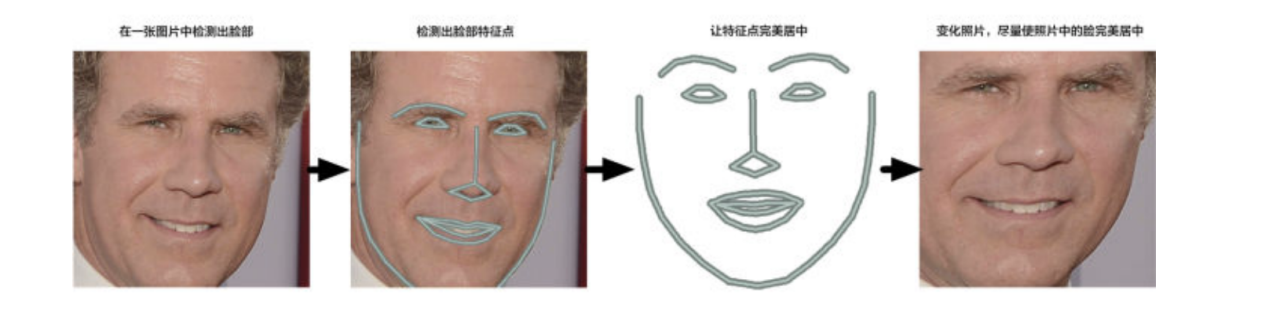
通过找到脸上的68个主要特征点,找出脸部的姿势。一旦我们找到这些特征点,就利用它们把图像扭曲,使眼睛和嘴巴居中。
通过使用称为面部特征点估计(face landmark estimation)的算法可以解决这一问题,基本思路:这一算法的基本思路是找到 68 个人脸上普遍存在的特定点(称为特征点, landmarks)——包括下巴的顶部、每只眼睛的外部轮廓、每条眉毛的内部轮廓等。接下来我们训练一个机器学习算法,让它能够在任何脸部找到这 68 个特定的点。

既然已经知道了眼睛和嘴巴在哪儿,接下来将图像进行旋转、缩放和错切,使得眼睛和嘴巴尽可能靠近中心。这里不会做任何花哨的三维扭曲,因为这会让图像失真。只会使用那些能够保持图片相对平行的基本图像变换,比如旋转和缩放(称为仿射变换):
3. 神经网络
现在进入到最关键的一部分内容,就是如何区分不同的人脸?
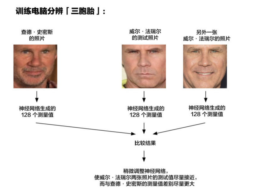
解决方案是训练一个深度卷积神经网络,但是,并不是让它去识别图片中的物体,这一次我们的训练是要让它为脸部生成 128 个测量值。
每次训练要观察三个不同的脸部图像:
一. 加载一张已知的人的面部训练图像

二. 加载同一个人的另一张照片

三. 加载另外一个人的照片
然后,算法查看它自己为这三个图片生成的测量值。再然后,稍微调整神经网络,以确保第一张和第二张生成的测量值接近,而第二张和第三张生成的测量值略有不同。
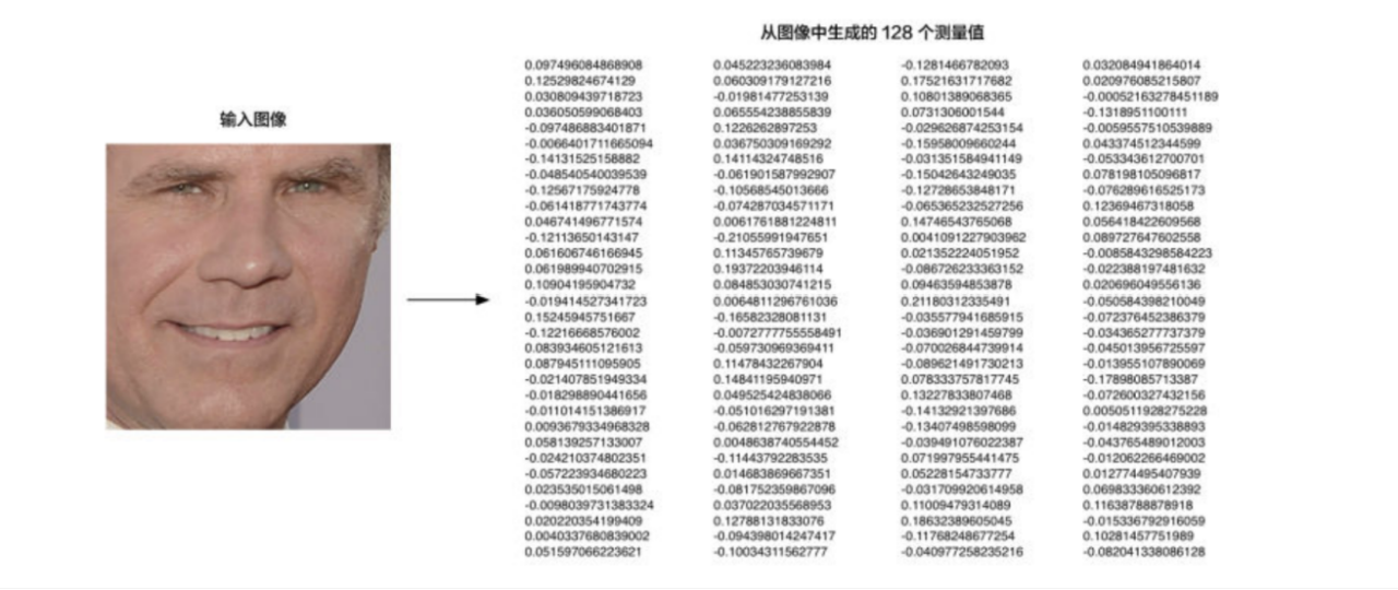
把上一步得到的面部图像放入神经网络中,神经网络知道如何找到 128 个特征测量值。保存这 128 个测量值。
在为几千个人的数百万图像重复该步骤数百万次之后,神经网络学习了如何可靠地为每个人生成 128 个测量值。对于同一个人的任何十张不同的照片,它都应该给出大致相同的测量值。 128个测试值对于我们来说,并不需要知道它们是什么东西,也不需要它们是如何计算出来的,这是计算机通过深度学习而得到的对它有意义的值。
4. 分类
看看我们过去已经测量过的所有脸部,找出哪个人的测量值和我们要测量的面部最接近。这一步相对简单,使用各类分类算法即可,下面有两种分类算法推荐。
k-means:k均值聚类算法(k-means clustering algorithm) 参考我的博客 https://www.cnblogs.com/UniqueColor/p/10996269.html
KNN:K最近邻(k-NearestNeighbor)参考我的博客 https://www.cnblogs.com/UniqueColor/p/10996331.html
四、演示(使用Face Recognition)
1、识别到照片上的所有人脸
 1 # -*- coding: utf-8 -*-
 2
 3 # 检测人脸
 4 import face_recognition
 5 import cv2
 6
 7 # 读取图片并识别人脸
 8 img = face_recognition.load_image_file("scl.jpg")
 9 face_locations = face_recognition.face_locations(img)
10 print(face_locations)
11
12 # 调用opencv函数显示图片
13 img = cv2.imread("scl.jpg")
14 # cv2.namedWindow("origin")
15 # cv2.imshow("origin", img)
16
17 # 遍历每个人脸,并标注
18 faceNum = len(face_locations)
19 for i in range(0, faceNum):
20     top = face_locations[i][0]
21     right = face_locations[i][1]
22     bottom = face_locations[i][2]
23     left = face_locations[i][3]
24
25     start = (left, top)
26     end = (right, bottom)
27
28     color = (55, 255, 155)
29     thickness = 3
30     cv2.rectangle(img, start, end, color, thickness)
31
32 # 显示识别结果
33 cv2.namedWindow("recognition")
34 cv2.imshow("recognition", img)
35
36 cv2.waitKey(0)
37 cv2.destroyAllWindows()
效果:

2、照片上识别人脸并且确定是哪个人
 1 # -*- coding: utf-8 -*-
 2
 3 import face_recognition
 4 from PIL import Image, ImageDraw
 5 import numpy as np
 6
 7
 8 # 加载数据源.
 9 klay_image = face_recognition.load_image_file("Klay_Thompson.jpg")
10 klay_face_encoding = face_recognition.face_encodings(klay_image)[0]
11
12 # 加载数据源.
13 curry_image = face_recognition.load_image_file("Stephen_Curry.jpg")
14 curry_face_encoding = face_recognition.face_encodings(curry_image)[0]
15
16 # 创建已知人脸编码及其名称的数组
17 known_face_encodings = [
18     klay_face_encoding,
19     curry_face_encoding
20 ]
21 known_face_names = [
22     "Klay Thompson",
23     "Stepthen Curry"
24 ]
25
26 # 加载要识别的图像
27 unknown_image = face_recognition.load_image_file("scl.jpg")
28
29 # 查找未知图像中所有的脸和脸编码
30 face_locations = face_recognition.face_locations(unknown_image)
31 face_encodings = face_recognition.face_encodings(unknown_image, face_locations)
32
33 # 将图像转换为PIL格式的图像,创建绘制实例
34 pil_image = Image.fromarray(unknown_image)
35 draw = ImageDraw.Draw(pil_image)
36
37 # 循环要识别的图像中的每一张脸
38 for (top, right, bottom, left), face_encoding in zip(face_locations, face_encodings):
39     # 看看这张脸是否与已知的脸匹配
40     matches = face_recognition.compare_faces(known_face_encodings, face_encoding)
41
42     name = "Unknown"
43
44
45     # 使用将要识别的脸与已知的脸作比较,计算出距离最小的脸
46     face_distances = face_recognition.face_distance(known_face_encodings, face_encoding)
47     best_match_index = np.argmin(face_distances)
48     if matches[best_match_index]:
49         name = known_face_names[best_match_index]
50
51     # 在面部周围绘制一个方框
52     draw.rectangle(((left, top), (right, bottom)), outline=(0, 0, 255))
53
54     # 在脸下绘制名称
55     text_width, text_height = draw.textsize(name)
56     draw.rectangle(((left, bottom - text_height - 10), (right, bottom)), fill=(0, 0, 255), outline=(0, 0, 255))
57     draw.text((left + 6, bottom - text_height - 5), name, fill=(255, 255, 255, 255))
58
59
60 del draw
61
62 # 展示结果
63 pil_image.show()
图片效果:

3、视频上实时识别人脸并且确定是哪个人
 1 # -*- coding: utf-8 -*-
 2 import face_recognition
 3 import cv2
 4
 5 # 打开视频
 6 input_movie = cv2.VideoCapture("hamilton_clip.mp4")
 7 length = int(input_movie.get(cv2.CAP_PROP_FRAME_COUNT))
 8
 9 # 创建输出的视频
10 fourcc = cv2.VideoWriter_fourcc(*'XVID')
11 output_movie = cv2.VideoWriter('output.mp4', fourcc, 29.97, (640, 360))
12
13 # # 加载数据源.
14 lmm_image = face_recognition.load_image_file("lin-manuel-miranda.png")
15 lmm_face_encoding = face_recognition.face_encodings(lmm_image)[0]
16
17 # 加载数据源.
18 curry_image = face_recognition.load_image_file("Stephen_Curry.jpg")
19 curry_face_encoding = face_recognition.face_encodings(curry_image)[0]
20
21 # 创建已知人脸编码及其名称的数组
22 known_face_encodings = [
23     lmm_face_encoding,
24     curry_face_encoding
25 ]
26
27
28 face_locations = []
29 face_encodings = []
30 face_names = []
31 frame_number = 0
32
33 while True:
34     # 抓取视频帧
35     ret, frame = input_movie.read()
36     frame_number += 1
37
38     # 抓取结束
39     if not ret:
40         break
41
42     # 将图像从bgr颜色(opencv使用)转换为rgb颜色(人脸识别使用)
43     rgb_frame = frame[:, :, ::-1]
44
45     # 找到视频中所有的人脸
46     face_locations = face_recognition.face_locations(rgb_frame)
47     face_encodings = face_recognition.face_encodings(rgb_frame, face_locations)
48
49     face_names = []
50     for face_encoding in face_encodings:
51         # 看看这张脸是否与已知的脸匹配
52         match = face_recognition.compare_faces(known_face_encodings, face_encoding, tolerance=0.50)
53
54         # 判断人脸逻辑
55         name = None
56         if match[0]:
57             name = "Lin-Manuel Miranda"
58         elif match[1]:
59             name = "Stepthen Curry"
60
61         face_names.append(name)
62
63     # 展示识别结果
64     for (top, right, bottom, left), name in zip(face_locations, face_names):
65         if not name:
66             continue
67
68         # 画框
69         cv2.rectangle(frame, (left, top), (right, bottom), (0, 0, 255), 2)
70
71         # 写上人名
72         cv2.rectangle(frame, (left, bottom - 25), (right, bottom), (0, 0, 255), cv2.FILLED)
73         font = cv2.FONT_HERSHEY_DUPLEX
74         cv2.putText(frame, name, (left + 6, bottom - 6), font, 0.5, (255, 255, 255), 1)
75
76     # 写入到结果视频中
77     print("Writing frame {} / {}".format(frame_number, length))
78     output_movie.write(frame)
79
80
81 input_movie.release()
82 cv2.destroyAllWindows()
视频由于比较大,就不做演示了,有兴趣可以自己试试。
五、手写神经网络
上文提到了神经网络,那么神经网络到底是什么?接下来就以一个简单的例子探探神经网络。
1. 神经元
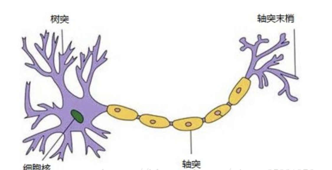
如图所示生物神经元包括细胞体,树突,轴突等部分。
树突是用于接受输入信息,输入信息经过突触处理,当达到一定条件时通过轴突传出,此时神经元处于激活状态;反之没有达到相应条件,则神经元处于抑制状态。
受到生物神经元的启发,于是神经网络模型就出来了。神经元是神经网络的基本组成部分,它获取到输入后,然后执行某些数学运算后,产生了输出。
如下所示,将神经元转化成数学图形
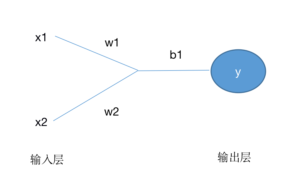
在这个神经元中,设x1、x2为输入,w1、w2为权重,b为偏置,
按照上图的数学运算有:
x1*w1+x2*w2+b
最后再经过激活函数处理得到:
y = f(x1 × w1 + x2 × w2 + b)
思考:为什么使用激活函数?
如果不使用激励函数(相当于激活函数是f(x) = x),在这种情况下你每一层节点的输入都是上层输出的线性函数,很容易验证,无论你神经网络有多少层,输出都是输入的线性组合,与没有隐藏层效果相当,这种情况就是最原始的感知机(Perceptron)了,那么神经网络的逼近能力就相当有限。
正因如此,引入非线性函数作为激励函数,这样深层神经网络表达能力就更加强大(不再是输入的线性组合,而是几乎可以逼近任意函数)。
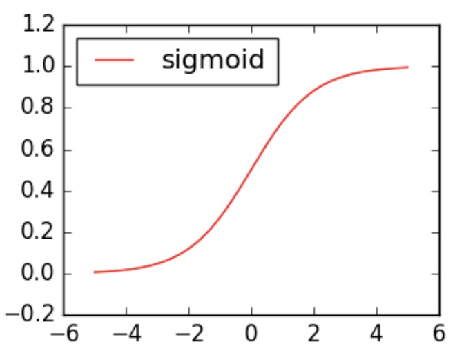
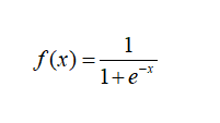
激活函数就是将无限制的输入转换为可预测形式的输出,输出介于0和1, 即把 (−∞,+∞) 范围内的数压缩到 (0, 1)以内。正值越大输出越接近1,负向数值越大输出越接近0。
2.搭建神经网络
神经网络其实就是若干神经元组成而来,如下:
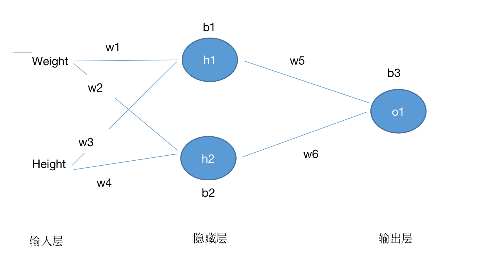
这个网络有2个输入、一个包含2个神经元的隐藏层(h1和h2)、包含1个神经元的输出层o1。
隐藏层是夹在输入输入层和输出层之间的部分,一个神经网络可以有多个隐藏层。
把神经元的输入向前传递获得输出的过程称为前馈(feedforward)。
即:
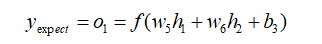
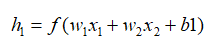
h1=f(x1 × w1 + x2 × w2 + b1)

h2=f(x1 × w3 + x2 × w4 + b2)

o1=f(h1 × w5 + h2 × w6 + b3)
3.训练神经网络
训练神经网络,其实是不断迭代优化的过程,可以理解为寻找最优解。
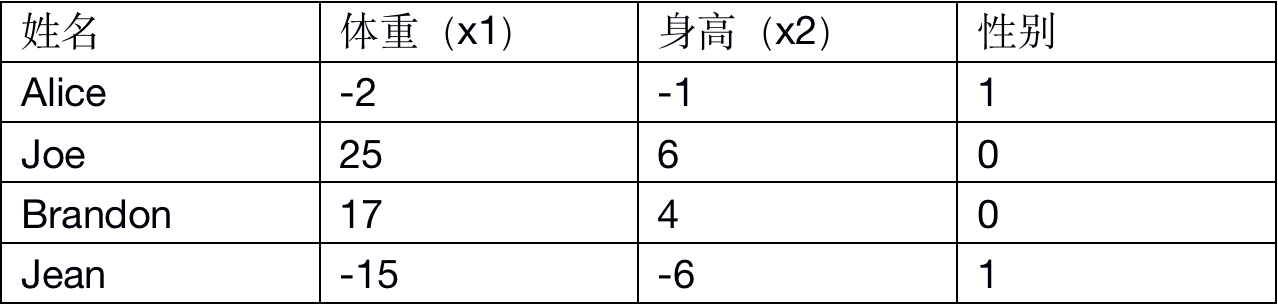
如:接下来的目标是通过某人的身高、体重预测这个人的性别。有如下的数据:
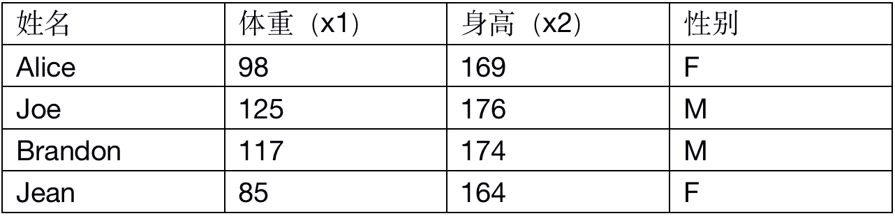
这里为了简便将每个人的身高、体重减去一个固定数值(体重-100,身高-170),性别男定义为0、性别女定义为1。
在训练神经网络之前,我们需要有一个标准定义它到底好不好,以便我们进行改进,这就是损失。
如用 均方误差 来定义损失:
公式①
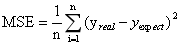
n是样本的数量,在上面的数据集中是4;
y代表人的性别,男性是0,女性是1;
y_real是变量的真实值,y_expect是变量的预测值。
均方误差就是所有数据方差的平均值(损失函数MSE)。预测结果越好,损失就越低,训练神经网络就是将损失最小化。
MSE= 1/4 [(1-0)^2+(0-0)^2+(0-0)^2+(1-0)^2]= 0.5
4. 减杀神经网络损失
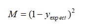
上面的结果一看就知道不够好,所以还需要不断的优化神经网络,减少损失。所以这里通过改变权重(w)和偏置(b)值可以影响神经网络的产出。为了方便计算,这里把数据集缩减到只剩下一个人的情况。
于是上述MSE的计算可简化成:
公式②

预测值是由一系列网络权重和偏置计算出来的:


所以损失函数实际上是包含多个权重、偏置的多元函数:
M(w1, w2, w3, w4, w5, w6, b1, b2, b3)

再由方差计算公式①②得:
公式④
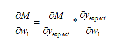
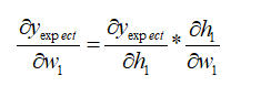
将④代入![]() ,以
,以 求导得:
求导得:
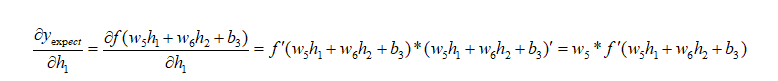
又根据神经元运算规则得:
公式⑥
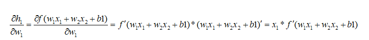
再由单个神经元可知h1与w1关系密切,所以再次使用链式法则得:
公式⑦
将⑥代入![]() 得
得
公式⑧
同样再次运行神经元运算法则得:
公式⑨
将上式代入到![]() 得
得
公式⑩
最后是激活函数的公式
公式⑪
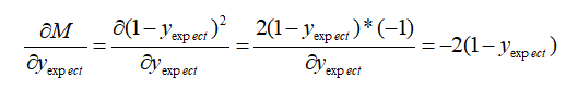
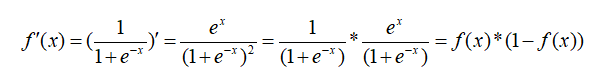
对激活函数⑪求导得:
公式⑫
综上,由③⑦得:
公式⑬
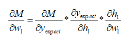
由⑬⑤⑧⑩得
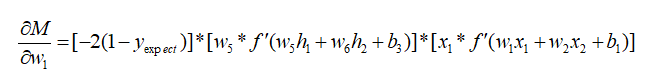
假设x1=-2,x2=-1,w1=w2=w3=w4=w5=w6=1,b1=b2=b3=0,代入神经元计算公式得:

o1=y(expect)=0.524这个值并不能强烈的预测是男是女,说明这个值还不够准确,接下来代入⑪⑫看看:
∂M/∂w1=0.0214,可得w1与M成正比,M随着w1增大而增加。
5、迭代优化
由上经过一次优化显示还不够,所以这里还需要再经过随机梯度下降法(SGD) 的迭代优化。
随机梯度下降(SGD)是每次迭代使用一个样本来对参数进行更新。使得训练速度加快。普通的BGD算法是每次迭代把所有样本都过一遍,每训练一组样本就把梯度更新一次。而SGD算法是从样本中随机抽出一组,训练后按梯度更新一次,然后再抽取一组,再更新一次,在样本量及其大的情况下,可能不用训练完所有的样本就可以获得一个损失值在可接受范围之内的模型了。
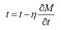
t表示变量, 表示变化率。通过不断修改变量值来达到降低损失(MES)的目的,从而达到神经网络的不断优化。
代码Demo(注意项目上的神经网络可没这么简单):
  1 import numpy as np
  2
  3 def sigmoid(x):
  4   # sigmoid激活函数: f(x) = 1 / (1 + e^(-x)),将无限制的输入转换为可预测形式的输出,输出介于0和1。
  5   # 即把 (−∞,+∞) 范围内的数压缩到 (0, 1)以内。正值越大输出越接近1,负向数值越大输出越接近0。
  6   return 1 / (1 + np.exp(-x))
  7
  8 def deriv_sigmoid(x):
  9   # 求激活函数的偏导数: f'(x) = f(x) * (1 - f(x))
 10   fx = sigmoid(x)
 11   return fx * (1 - fx)
 12
 13 def mse_loss(y_real, y_expect):
 14   # 计算损失函数,其实就是所有数据方差的平均值(均方误差),预测结果越好,损失就越低,训练神经网络就是将损失最小化
 15   # y_real 和 y_expect 是同样长度的数组.
 16   return ((y_real - y_expect) ** 2).mean()
 17
 18 class NeuralNetworkDemo:
 19   '''
 20   一个神经网络包括:
 21     - 2个输入
 22     - 1个有2 个神经元 (h1, h2)的隐藏层
 23     - 一个神经元的输出层 (o1)
 24   '''
 25   def __init__(self):
 26     # 随机初始化权重值
 27     self.w1 = np.random.normal()
 28     self.w2 = np.random.normal()
 29     self.w3 = np.random.normal()
 30     self.w4 = np.random.normal()
 31     self.w5 = np.random.normal()
 32     self.w6 = np.random.normal()
 33
 34     # 随机初始化偏置值
 35     self.b1 = np.random.normal()
 36     self.b2 = np.random.normal()
 37     self.b3 = np.random.normal()
 38
 39   def feedforward(self, x):
 40     # x包含x[0]、x[1],计算前馈:神经元的输入向前传递获得输出的过程
 41     h1 = sigmoid(self.w1 * x[0] + self.w2 * x[1] + self.b1)
 42     h2 = sigmoid(self.w3 * x[0] + self.w4 * x[1] + self.b2)
 43     o1 = sigmoid(self.w5 * h1 + self.w6 * h2 + self.b3)
 44     return o1
 45
 46   # 训练过程:
 47   # 1、从数据集中选择一个样本;
 48   # 2、计算损失函数对所有权重和偏置的偏导数;
 49   # 3、使用更新公式更新每个权重和偏置;
 50   # 4、回到第1步。
 51   def train(self, data, all_y_reals):
 52     '''
 53     - data is a (n x 2) numpy array, n = # of samples in the dataset.
 54     - all_y_reals is a numpy array with n elements.
 55       Elements in all_y_reals correspond to those in data.
 56     '''
 57     learn_rate = 0.1
 58
 59     # 循环遍历整个数据集的次数
 60     iterations = 1000
 61
 62     for iteration in range(iterations):
 63       for x, y_real in zip(data, all_y_reals):
 64         # 计算h1的前馈
 65         sum_h1 = self.w1 * x[0] + self.w2 * x[1] + self.b1
 66         h1 = sigmoid(sum_h1)
 67
 68         # 计算h2的前馈
 69         sum_h2 = self.w3 * x[0] + self.w4 * x[1] + self.b2
 70         h2 = sigmoid(sum_h2)
 71
 72         # 计算o1的前馈
 73         sum_o1 = self.w5 * h1 + self.w6 * h2 + self.b3
 74         o1 = sigmoid(sum_o1)
 75         y_expect = o1
 76
 77         # --- 计算部分偏导数
 78         # --- d_L_d_w1 表示 "偏导数 L / 偏导数 w1"
 79         d_L_d_ypred = -2 * (y_real - y_expect)
 80
 81         # 神经元 o1
 82         d_ypred_d_w5 = h1 * deriv_sigmoid(sum_o1)
 83         d_ypred_d_w6 = h2 * deriv_sigmoid(sum_o1)
 84         d_ypred_d_b3 = deriv_sigmoid(sum_o1)
 85
 86         d_ypred_d_h1 = self.w5 * deriv_sigmoid(sum_o1)
 87         d_ypred_d_h2 = self.w6 * deriv_sigmoid(sum_o1)
 88
 89         # 神经元 h1
 90         d_h1_d_w1 = x[0] * deriv_sigmoid(sum_h1)
 91         d_h1_d_w2 = x[1] * deriv_sigmoid(sum_h1)
 92         d_h1_d_b1 = deriv_sigmoid(sum_h1)
 93
 94         # 神经元 h2
 95         d_h2_d_w3 = x[0] * deriv_sigmoid(sum_h2)
 96         d_h2_d_w4 = x[1] * deriv_sigmoid(sum_h2)
 97         d_h2_d_b2 = deriv_sigmoid(sum_h2)
 98
 99         # --- 更新权重值和偏置值
100         # 神经元 h1
101         self.w1 -= learn_rate * d_L_d_ypred * d_ypred_d_h1 * d_h1_d_w1
102         self.w2 -= learn_rate * d_L_d_ypred * d_ypred_d_h1 * d_h1_d_w2
103         self.b1 -= learn_rate * d_L_d_ypred * d_ypred_d_h1 * d_h1_d_b1
104
105         # 神经元 h2
106         self.w3 -= learn_rate * d_L_d_ypred * d_ypred_d_h2 * d_h2_d_w3
107         self.w4 -= learn_rate * d_L_d_ypred * d_ypred_d_h2 * d_h2_d_w4
108         self.b2 -= learn_rate * d_L_d_ypred * d_ypred_d_h2 * d_h2_d_b2
109
110         # 神经元 o1
111         self.w5 -= learn_rate * d_L_d_ypred * d_ypred_d_w5
112         self.w6 -= learn_rate * d_L_d_ypred * d_ypred_d_w6
113         self.b3 -= learn_rate * d_L_d_ypred * d_ypred_d_b3
114
115       # 每一次循环计算总的损失 --- Calculate total loss at the end of each iteration
116       if iteration % 10 == 0:
117         y_expects = np.apply_along_axis(self.feedforward, 1, data)
118         loss = mse_loss(all_y_reals, y_expects)
119         print("Iteration %d Mes loss: %.3f" % (iteration, loss))
120
121 # 定义数据集
122 data = np.array([
123   [-2, -1],
124   [25, 6],
125   [17, 4],
126   [-15, -6],
127 ])
128 all_y_reals = np.array([
129   1,
130   0,
131   0,
132   1,
133 ])
134
135 # 训练神经网络
136 network = NeuralNetworkDemo()
137 network.train(data, all_y_reals)
运行结果:
Iteration 0 Mes loss: 0.335
Iteration 10 Mes loss: 0.205
Iteration 20 Mes loss: 0.128
Iteration 30 Mes loss: 0.087
Iteration 40 Mes loss: 0.063
Iteration 50 Mes loss: 0.049
Iteration 60 Mes loss: 0.039
Iteration 70 Mes loss: 0.032
Iteration 80 Mes loss: 0.028
Iteration 90 Mes loss: 0.024
Iteration 100 Mes loss: 0.021
Iteration 110 Mes loss: 0.019
Iteration 120 Mes loss: 0.017
Iteration 130 Mes loss: 0.015
Iteration 140 Mes loss: 0.014
Iteration 150 Mes loss: 0.013
Iteration 160 Mes loss: 0.012
Iteration 170 Mes loss: 0.011
Iteration 180 Mes loss: 0.010
Iteration 190 Mes loss: 0.010
Iteration 200 Mes loss: 0.009
Iteration 210 Mes loss: 0.009
Iteration 220 Mes loss: 0.008
Iteration 230 Mes loss: 0.008
Iteration 240 Mes loss: 0.007
Iteration 250 Mes loss: 0.007
Iteration 260 Mes loss: 0.007
Iteration 270 Mes loss: 0.006
Iteration 280 Mes loss: 0.006
Iteration 290 Mes loss: 0.006
Iteration 300 Mes loss: 0.006
Iteration 310 Mes loss: 0.005
Iteration 320 Mes loss: 0.005
Iteration 330 Mes loss: 0.005
Iteration 340 Mes loss: 0.005
Iteration 350 Mes loss: 0.005
Iteration 360 Mes loss: 0.005
Iteration 370 Mes loss: 0.004
Iteration 380 Mes loss: 0.004
Iteration 390 Mes loss: 0.004
Iteration 400 Mes loss: 0.004
Iteration 410 Mes loss: 0.004
Iteration 420 Mes loss: 0.004
Iteration 430 Mes loss: 0.004
Iteration 440 Mes loss: 0.004
Iteration 450 Mes loss: 0.004
Iteration 460 Mes loss: 0.003
Iteration 470 Mes loss: 0.003
Iteration 480 Mes loss: 0.003
Iteration 490 Mes loss: 0.003
Iteration 500 Mes loss: 0.003
Iteration 510 Mes loss: 0.003
Iteration 520 Mes loss: 0.003
Iteration 530 Mes loss: 0.003
Iteration 540 Mes loss: 0.003
Iteration 550 Mes loss: 0.003
Iteration 560 Mes loss: 0.003
Iteration 570 Mes loss: 0.003
Iteration 580 Mes loss: 0.003
Iteration 590 Mes loss: 0.003
Iteration 600 Mes loss: 0.003
Iteration 610 Mes loss: 0.003
Iteration 620 Mes loss: 0.002
Iteration 630 Mes loss: 0.002
Iteration 640 Mes loss: 0.002
Iteration 650 Mes loss: 0.002
Iteration 660 Mes loss: 0.002
Iteration 670 Mes loss: 0.002
Iteration 680 Mes loss: 0.002
Iteration 690 Mes loss: 0.002
Iteration 700 Mes loss: 0.002
Iteration 710 Mes loss: 0.002
Iteration 720 Mes loss: 0.002
Iteration 730 Mes loss: 0.002
Iteration 740 Mes loss: 0.002
Iteration 750 Mes loss: 0.002
Iteration 760 Mes loss: 0.002
Iteration 770 Mes loss: 0.002
Iteration 780 Mes loss: 0.002
Iteration 790 Mes loss: 0.002
Iteration 800 Mes loss: 0.002
Iteration 810 Mes loss: 0.002
Iteration 820 Mes loss: 0.002
Iteration 830 Mes loss: 0.002
Iteration 840 Mes loss: 0.002
Iteration 850 Mes loss: 0.002
Iteration 860 Mes loss: 0.002
Iteration 870 Mes loss: 0.002
Iteration 880 Mes loss: 0.002
Iteration 890 Mes loss: 0.002
Iteration 900 Mes loss: 0.002
Iteration 910 Mes loss: 0.002
Iteration 920 Mes loss: 0.002
Iteration 930 Mes loss: 0.002
Iteration 940 Mes loss: 0.002
Iteration 950 Mes loss: 0.002
Iteration 960 Mes loss: 0.002
Iteration 970 Mes loss: 0.002
Iteration 980 Mes loss: 0.002
Iteration 990 Mes loss: 0.001
可以看出随着迭代的不断进行,损失越来越小。
接下来可以使用自定义输入来预测性别了
 1 import numpy as np
 2
 3 def sigmoid(x):
 4   ..........
 5
 6 def deriv_sigmoid(x):
 7   ..........
 8
 9 def mse_loss(y_real, y_expect):
10   ..........
11
12 class NeuralNetworkDemo:
13   ..........
14
15   def testPredict(self):
16     you = np.array([-10, -10]) # 体重90,身高160。对于x1=90-100=-10,x2=160-170=-10
17     print("your output is ", network.feedforward(you))
18
19 # 定义数据集
20 ..........
21
22 # 训练神经网络
23 ..........
24 network.testPredict()
取一个体重90,身高160的女生来测试,输出结果为:
your output is 0.9651728303105593
不断执行多少次,其输出结果都接近于1,所以可以预测这是女生。
关于神经网络还有其它延伸及应用较广泛的类型(CNN、RNN、DBN、GAN等),有兴趣可以来探讨。