忙了许久,总算是又想起这边还没写完呢。
那今天就写写sklearn库的一部分简单内容吧,包括数据集调用,聚类,轮廓系数等等。
自带数据集API
| 数据集函数 | 中文翻译 | 任务类型 | 数据规模 |
|---|---|---|---|
| load_boston | Boston房屋价格 | 回归 | 506*13 |
| fetch_california_housing | 加州住房 | 回归 | 20640*9 |
| load_diabetes | 糖尿病 | 回归 | 442*10 |
| load_digits | 手写字 | 分类 | 1797*64 |
| load_breast_cancer | 乳腺癌 | 分类、聚类 | (357+212)*30 |
| load_iris | 鸢尾花 | 分类、聚类 | (50*3)*4 |
| load_wine | 葡萄酒 | 分类 | (59+71+48)*13 |
| load_linnerud | 体能训练 | 多分类 | 20 |
提取信息关键字:
- DESCR:数据集的描述信息
- data:内部数据
- feature_names:数据字段名
- target:数据标签
- target_names:标签字段名(回归数据集无此项)
开始提取
以load_iris为例。
# 导入是必须的
from sklearn.datasets import load_iris
iris = load_iris()
iris # iris的所有信息,包括数据集、标签集、各字段名等
这个输出太长太乱,而且后边也有,我就不复制过来了
iris.keys() # 数据集关键字
dict_keys(['data', 'target', 'target_names', 'DESCR', 'feature_names'])
descr = iris['DESCR']
data = iris['data']
feature_names = iris['feature_names']
target = iris['target']
target_names = iris['target_names']
descr
'Iris Plants Database ==================== Notes ----- Data Set Characteristics: :Number of Instances: 150 (50 in each of three classes) :Number of Attributes: 4 numeric, predictive attributes and the class :Attribute Information: - sepal length in cm - sepal width in cm - petal length in cm - petal width in cm - class: - Iris-Setosa - Iris-Versicolour - Iris-Virginica :Summary Statistics: ============== ==== ==== ======= ===== ==================== Min Max Mean SD Class Correlation ============== ==== ==== ======= ===== ==================== sepal length: 4.3 7.9 5.84 0.83 0.7826 sepal 2.0 4.4 3.05 0.43 -0.4194 petal length: 1.0 6.9 3.76 1.76 0.9490 (high!) petal 0.1 2.5 1.20 0.76 0.9565 (high!) ============== ==== ==== ======= ===== ==================== :Missing Attribute Values: None :Class Distribution: 33.3% for each of 3 classes. :Creator: R.A. Fisher :Donor: Michael Marshall (MARSHALL%PLU@io.arc.nasa.gov) :Date: July, 1988 This is a copy of UCI ML iris datasets. http://archive.ics.uci.edu/ml/datasets/Iris The famous Iris database, first used by Sir R.A Fisher This is perhaps the best known database to be found in the pattern recognition literature. Fisher's paper is a classic in the field and is referenced frequently to this day. (See Duda & Hart, for example.) The data set contains 3 classes of 50 instances each, where each class refers to a type of iris plant. One class is linearly separable from the other 2; the latter are NOT linearly separable from each other. References ---------- - Fisher,R.A. "The use of multiple measurements in taxonomic problems" Annual Eugenics, 7, Part II, 179-188 (1936); also in "Contributions to Mathematical Statistics" (John Wiley, NY, 1950). - Duda,R.O., & Hart,P.E. (1973) Pattern Classification and Scene Analysis. (Q327.D83) John Wiley & Sons. ISBN 0-471-22361-1. See page 218. - Dasarathy, B.V. (1980) "Nosing Around the Neighborhood: A New System Structure and Classification Rule for Recognition in Partially Exposed Environments". IEEE Transactions on Pattern Analysis and Machine Intelligence, Vol. PAMI-2, No. 1, 67-71. - Gates, G.W. (1972) "The Reduced Nearest Neighbor Rule". IEEE Transactions on Information Theory, May 1972, 431-433. - See also: 1988 MLC Proceedings, 54-64. Cheeseman et al"s AUTOCLASS II conceptual clustering system finds 3 classes in the data. - Many, many more ... '
data
array([[5.1, 3.5, 1.4, 0.2],
[4.9, 3. , 1.4, 0.2],
[4.7, 3.2, 1.3, 0.2],
[4.6, 3.1, 1.5, 0.2],
[5. , 3.6, 1.4, 0.2],
[5.4, 3.9, 1.7, 0.4],
[4.6, 3.4, 1.4, 0.3],
[5. , 3.4, 1.5, 0.2],
[4.4, 2.9, 1.4, 0.2],
[4.9, 3.1, 1.5, 0.1],
[5.4, 3.7, 1.5, 0.2],
[4.8, 3.4, 1.6, 0.2],
[4.8, 3. , 1.4, 0.1],
[4.3, 3. , 1.1, 0.1],
[5.8, 4. , 1.2, 0.2],
[5.7, 4.4, 1.5, 0.4],
[5.4, 3.9, 1.3, 0.4],
[5.1, 3.5, 1.4, 0.3],
[5.7, 3.8, 1.7, 0.3],
[5.1, 3.8, 1.5, 0.3],
[5.4, 3.4, 1.7, 0.2],
[5.1, 3.7, 1.5, 0.4],
[4.6, 3.6, 1. , 0.2],
[5.1, 3.3, 1.7, 0.5],
[4.8, 3.4, 1.9, 0.2],
[5. , 3. , 1.6, 0.2],
[5. , 3.4, 1.6, 0.4],
[5.2, 3.5, 1.5, 0.2],
[5.2, 3.4, 1.4, 0.2],
[4.7, 3.2, 1.6, 0.2],
[4.8, 3.1, 1.6, 0.2],
[5.4, 3.4, 1.5, 0.4],
[5.2, 4.1, 1.5, 0.1],
[5.5, 4.2, 1.4, 0.2],
[4.9, 3.1, 1.5, 0.1],
[5. , 3.2, 1.2, 0.2],
[5.5, 3.5, 1.3, 0.2],
[4.9, 3.1, 1.5, 0.1],
[4.4, 3. , 1.3, 0.2],
[5.1, 3.4, 1.5, 0.2],
[5. , 3.5, 1.3, 0.3],
[4.5, 2.3, 1.3, 0.3],
[4.4, 3.2, 1.3, 0.2],
[5. , 3.5, 1.6, 0.6],
[5.1, 3.8, 1.9, 0.4],
[4.8, 3. , 1.4, 0.3],
[5.1, 3.8, 1.6, 0.2],
[4.6, 3.2, 1.4, 0.2],
[5.3, 3.7, 1.5, 0.2],
[5. , 3.3, 1.4, 0.2],
[7. , 3.2, 4.7, 1.4],
[6.4, 3.2, 4.5, 1.5],
[6.9, 3.1, 4.9, 1.5],
[5.5, 2.3, 4. , 1.3],
[6.5, 2.8, 4.6, 1.5],
[5.7, 2.8, 4.5, 1.3],
[6.3, 3.3, 4.7, 1.6],
[4.9, 2.4, 3.3, 1. ],
[6.6, 2.9, 4.6, 1.3],
[5.2, 2.7, 3.9, 1.4],
[5. , 2. , 3.5, 1. ],
[5.9, 3. , 4.2, 1.5],
[6. , 2.2, 4. , 1. ],
[6.1, 2.9, 4.7, 1.4],
[5.6, 2.9, 3.6, 1.3],
[6.7, 3.1, 4.4, 1.4],
[5.6, 3. , 4.5, 1.5],
[5.8, 2.7, 4.1, 1. ],
[6.2, 2.2, 4.5, 1.5],
[5.6, 2.5, 3.9, 1.1],
[5.9, 3.2, 4.8, 1.8],
[6.1, 2.8, 4. , 1.3],
[6.3, 2.5, 4.9, 1.5],
[6.1, 2.8, 4.7, 1.2],
[6.4, 2.9, 4.3, 1.3],
[6.6, 3. , 4.4, 1.4],
[6.8, 2.8, 4.8, 1.4],
[6.7, 3. , 5. , 1.7],
[6. , 2.9, 4.5, 1.5],
[5.7, 2.6, 3.5, 1. ],
[5.5, 2.4, 3.8, 1.1],
[5.5, 2.4, 3.7, 1. ],
[5.8, 2.7, 3.9, 1.2],
[6. , 2.7, 5.1, 1.6],
[5.4, 3. , 4.5, 1.5],
[6. , 3.4, 4.5, 1.6],
[6.7, 3.1, 4.7, 1.5],
[6.3, 2.3, 4.4, 1.3],
[5.6, 3. , 4.1, 1.3],
[5.5, 2.5, 4. , 1.3],
[5.5, 2.6, 4.4, 1.2],
[6.1, 3. , 4.6, 1.4],
[5.8, 2.6, 4. , 1.2],
[5. , 2.3, 3.3, 1. ],
[5.6, 2.7, 4.2, 1.3],
[5.7, 3. , 4.2, 1.2],
[5.7, 2.9, 4.2, 1.3],
[6.2, 2.9, 4.3, 1.3],
[5.1, 2.5, 3. , 1.1],
[5.7, 2.8, 4.1, 1.3],
[6.3, 3.3, 6. , 2.5],
[5.8, 2.7, 5.1, 1.9],
[7.1, 3. , 5.9, 2.1],
[6.3, 2.9, 5.6, 1.8],
[6.5, 3. , 5.8, 2.2],
[7.6, 3. , 6.6, 2.1],
[4.9, 2.5, 4.5, 1.7],
[7.3, 2.9, 6.3, 1.8],
[6.7, 2.5, 5.8, 1.8],
[7.2, 3.6, 6.1, 2.5],
[6.5, 3.2, 5.1, 2. ],
[6.4, 2.7, 5.3, 1.9],
[6.8, 3. , 5.5, 2.1],
[5.7, 2.5, 5. , 2. ],
[5.8, 2.8, 5.1, 2.4],
[6.4, 3.2, 5.3, 2.3],
[6.5, 3. , 5.5, 1.8],
[7.7, 3.8, 6.7, 2.2],
[7.7, 2.6, 6.9, 2.3],
[6. , 2.2, 5. , 1.5],
[6.9, 3.2, 5.7, 2.3],
[5.6, 2.8, 4.9, 2. ],
[7.7, 2.8, 6.7, 2. ],
[6.3, 2.7, 4.9, 1.8],
[6.7, 3.3, 5.7, 2.1],
[7.2, 3.2, 6. , 1.8],
[6.2, 2.8, 4.8, 1.8],
[6.1, 3. , 4.9, 1.8],
[6.4, 2.8, 5.6, 2.1],
[7.2, 3. , 5.8, 1.6],
[7.4, 2.8, 6.1, 1.9],
[7.9, 3.8, 6.4, 2. ],
[6.4, 2.8, 5.6, 2.2],
[6.3, 2.8, 5.1, 1.5],
[6.1, 2.6, 5.6, 1.4],
[7.7, 3. , 6.1, 2.3],
[6.3, 3.4, 5.6, 2.4],
[6.4, 3.1, 5.5, 1.8],
[6. , 3. , 4.8, 1.8],
[6.9, 3.1, 5.4, 2.1],
[6.7, 3.1, 5.6, 2.4],
[6.9, 3.1, 5.1, 2.3],
[5.8, 2.7, 5.1, 1.9],
[6.8, 3.2, 5.9, 2.3],
[6.7, 3.3, 5.7, 2.5],
[6.7, 3. , 5.2, 2.3],
[6.3, 2.5, 5. , 1.9],
[6.5, 3. , 5.2, 2. ],
[6.2, 3.4, 5.4, 2.3],
[5.9, 3. , 5.1, 1.8]])
feature_names
['sepal length (cm)',
'sepal width (cm)',
'petal length (cm)',
'petal width (cm)']
target
array([0, 0, 0, 0, 0, 0, 0, 0, 0, 0, 0, 0, 0, 0, 0, 0, 0, 0, 0, 0, 0, 0,
0, 0, 0, 0, 0, 0, 0, 0, 0, 0, 0, 0, 0, 0, 0, 0, 0, 0, 0, 0, 0, 0,
0, 0, 0, 0, 0, 0, 1, 1, 1, 1, 1, 1, 1, 1, 1, 1, 1, 1, 1, 1, 1, 1,
1, 1, 1, 1, 1, 1, 1, 1, 1, 1, 1, 1, 1, 1, 1, 1, 1, 1, 1, 1, 1, 1,
1, 1, 1, 1, 1, 1, 1, 1, 1, 1, 1, 1, 2, 2, 2, 2, 2, 2, 2, 2, 2, 2,
2, 2, 2, 2, 2, 2, 2, 2, 2, 2, 2, 2, 2, 2, 2, 2, 2, 2, 2, 2, 2, 2,
2, 2, 2, 2, 2, 2, 2, 2, 2, 2, 2, 2, 2, 2, 2, 2, 2, 2])
target_names
array(['setosa', 'versicolor', 'virginica'], dtype='<U10')
小试一下
from sklearn.cluster import KMeans  # 聚类包
from sklearn.preprocessing import StandardScaler, MinMaxScaler  # 预处理包
# 标准差标准化
# 公式:(x-mean(X))/std(X)
scale = StandarScaler().fit(data)  # 训练规则
X = scale.transform(data)  # 应用规则
# 离差标准化(零一标准化)
# 公式:(x-min(X))/(max(X)-min(X))
scale = MinMaxScaler().fit(data) # 训练规则
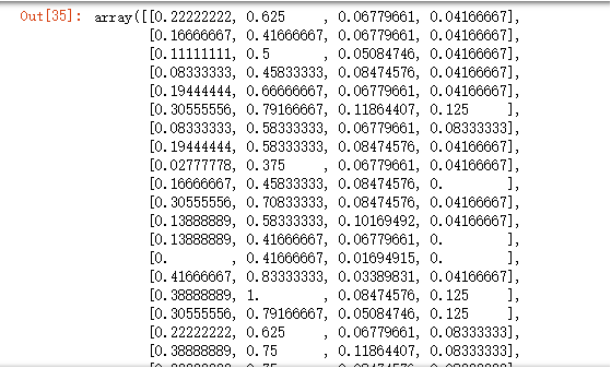
X = scale.transform(data) # 应用规则
X
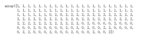
clf = KMeans(n_clusters = 3, random_state = 123).fit(X)  # 聚成3类
clf.labels_
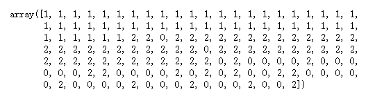
kmeans = KMeans(n_clusters = 3, random_state = 123).fit(data)  # 用data对比一下
kmeans.labels_
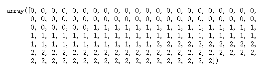
target # 这里我们也可以再拿出原始标签相互对比
当然啦,先人们也是一早就想着:得找个办法来衡量一下聚类效果啊。
于是乎,轮廓系数就诞生了。
且看下方代码。
'''这里插入一下轮廓系数的一些知识点吧
1.对于第i个对象,计算它到所属簇中所有其他对象的平均距离,记ai(体现凝聚度)
2.对于第i个对象和不包含该对象的任意簇,计算该对象到给定簇中所有对象的平均距离,取最小,记bi(体现分离度)
3.第i个对象的轮廓系数为si=(bi-ai)/max(ai, bi)
所以,很明显:轮廓系数取值为[-1,1],且越大越好;若值为负,即ai>bi,说明样本被分配到错误的簇中,不可接受;若值接近0,ai≈bi,表明聚类结果有重叠的情况。
'''
from sklearn.metrics import silhouette_score # 轮廓系数
import matplotlib.pyplot as plt
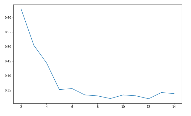
silhouettteScore = []
for i in range(2,15):
kmeans = KMeans(n_clusters = i,random_state=123).fit(X) ##构建并训练模型
score = silhouette_score(X,kmeans.labels_) # X是零一化之后的数据
silhouettteScore.append(score)
plt.figure(figsize=(10,6))
plt.plot(range(2,15),silhouettteScore,linewidth=1.5, linestyle="-")
plt.show()
嗯,到此先结束吧,等下一篇我们再继续讲构建回归模型。