机器学习相关知识汇总

1、算法模型

      算法模型对象:特殊的对象.在该对象中已经集成好个一个方程(还没有求出解的方程).

    - 模型对象的作用:通过方程实现预测或者分类

    - 样本数据(df,np):

•  特征数据:自变量
•  目标数据:因变量

2、模型对象的分类

    - 有监督学习:模型需要的样本数据中存在特征数据和目标数据
    - 无监督学习:模型需要的样本数据中存在特征数据
    - 半监督学习:模型需要的样本数据部分需要有特征数据和目标数据,部分只需要特征数据

3、sklearn模块

        sklearn模块封装了多种算法模型对象.
        导入sklearn，建立线性回归算法模型对象

      sklearn 模块开发流程：

           1、实例模型对象
           2、获取样本数据
           3、训练模型
           4、测试结果

 利用sklearn模块 实现预测，处理流程如下：

              注意： .reshape(-1,1) 将一维数组变为二维数组(将行变为列)

                          plt.scatter() 绘图

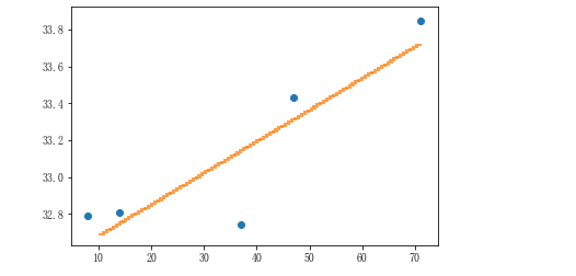
#1.导包
from sklearn.linear_model import LinearRegression
import matplotlib.pyplot as plt
%matplotlib inline

#2.实例化模型对象
linner = LinearRegression()
#3.提取样本数据:必须是二维数组 numpy或dataFrame
#4.训练模型:往方程里带数据求出方程式 linner.fit(x[],y[])
linner.fit(near_city_dist.reshape(-1,1),near_city_max_temp)
#5.实现预测:带入x求y
linner.predict(38) 
#array([33.16842645])

#6.给模型打分--大概值
linner.score(near_city_dist.reshape(-1,1),near_city_max_temp)
0.77988083971852
 
# 7.绘制回归曲线
x = np.linspace(10,70,num=100)
y = linner.predict(x.reshape(-1,1))
 
plt.scatter(near_city_dist,near_city_max_temp)# 
plt.scatter(x,y,s=0.2)

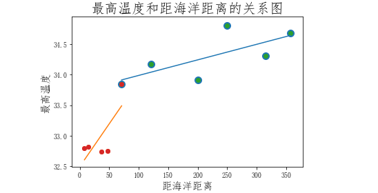
#将近海和远海的散点图合并显示
plt.scatter(far_city_dists,far_max_temps,s=100)
plt.scatter(near_city_dists,near_max_temps)
plt.scatter(far_city_dists,far_max_temps)
plt.plot(x,y)
plt.scatter(near_city_dists,near_max_temps)
plt.plot(x1,y1)
plt.title('最高温度和距海洋距离的关系图',fontsize=20)
plt.xlabel('距海洋距离',fontsize=15)
plt.ylabel('最高温度',fontsize=15)

 

 scatter函数的用法：绘制散点图

 plot() 函数的用法：画线图

未完待续.........

相关文章：

对于线性回归通俗理解的笔记  https://www.cnblogs.com/aitree/p/14324669.html