1.搭建神经网络基本流程

定义添加神经层的函数

1.训练的数据
2.定义节点准备接收数据
3.定义神经层：隐藏层和预测层
4.定义 loss 表达式
5.选择 optimizer 使 loss 达到最小

然后对所有变量进行初始化，通过 sess.run optimizer，迭代 1000 次进行学习：

import tensorflow as tf
import numpy as np

# 添加层
def add_layer(inputs, in_size, out_size, activation_function=None):
    # add one more layer and return the output of this layer
    Weights = tf.Variable(tf.random_normal([in_size, out_size]))
    biases = tf.Variable(tf.zeros([1, out_size]) + 0.1)
    Wx_plus_b = tf.matmul(inputs, Weights) + biases
    if activation_function is None:
        outputs = Wx_plus_b
    else:
        outputs = activation_function(Wx_plus_b)
    return outputs

# 1.训练的数据
# Make up some real data 
x_data = np.linspace(-1,1,300)[:, np.newaxis]
noise = np.random.normal(0, 0.05, x_data.shape)
y_data = np.square(x_data) - 0.5 + noise

# 2.定义节点准备接收数据
# define placeholder for inputs to network  
xs = tf.placeholder(tf.float32, [None, 1])
ys = tf.placeholder(tf.float32, [None, 1])

# 3.定义神经层：隐藏层和预测层
# add hidden layer 输入值是 xs，在隐藏层有 10 个神经元   
l1 = add_layer(xs, 1, 10, activation_function=tf.nn.relu)
# add output layer 输入值是隐藏层 l1，在预测层输出 1 个结果
prediction = add_layer(l1, 10, 1, activation_function=None)

# 4.定义 loss 表达式
# the error between prediciton and real data    
loss = tf.reduce_mean(tf.reduce_sum(tf.square(ys - prediction),
                     reduction_indices=[1]))

# 5.选择 optimizer 使 loss 达到最小                   
# 这一行定义了用什么方式去减少 loss，学习率是 0.1       
train_step = tf.train.GradientDescentOptimizer(0.1).minimize(loss)


# important step 对所有变量进行初始化
init = tf.initialize_all_variables()
sess = tf.Session()
# 上面定义的都没有运算，直到 sess.run 才会开始运算
sess.run(init)

# 迭代 1000 次学习，sess.run optimizer
for i in range(1000):
    # training train_step 和 loss 都是由 placeholder 定义的运算，所以这里要用 feed 传入参数
    sess.run(train_step, feed_dict={xs: x_data, ys: y_data})
    if i % 50 == 0:
        # to see the step improvement
        print(sess.run(loss, feed_dict={xs: x_data, ys: y_data}))

2. 主要步骤的解释：

• 之前写过一篇文章 TensorFlow 入门 讲了 tensorflow 的安装，这里使用时直接导入：

  import tensorflow as tf
  import numpy as np

• 导入或者随机定义训练的数据 x 和 y：

x_data = np.random.rand(100).astype(np.float32)
y_data = x_data*0.1 + 0.3

• 先定义出参数 Weights，biases，拟合公式 y，误差公式 loss：

Weights = tf.Variable(tf.random_uniform([1], -1.0, 1.0))
biases = tf.Variable(tf.zeros([1]))
y = Weights*x_data + biases
loss = tf.reduce_mean(tf.square(y-y_data))

• 选择 Gradient Descent 这个最基本的 Optimizer：

optimizer = tf.train.GradientDescentOptimizer(0.5)

• 神经网络的 key idea，就是让 loss 达到最小：

train = optimizer.minimize(loss)

• 前面是定义，在运行模型前先要初始化所有变量：

init = tf.initialize_all_variables()

• 接下来把结构激活，sesseion像一个指针指向要处理的地方：

sess = tf.Session()

• init 就被激活了，不要忘记激活：

sess.run(init)

• 训练201步：

for step in range(201):

• 要训练 train，也就是 optimizer：

sess.run(train)

• 每 20 步打印一下结果，sess.run 指向 Weights，biases 并被输出：

if step % 20 == 0:
print(step, sess.run(Weights), sess.run(biases))

所以关键的就是 y，loss，optimizer 是如何定义的。

3. TensorFlow 基本概念及代码：

在 TensorFlow 入门 也提到了几个基本概念，这里是几个常见的用法。

• Session

矩阵乘法：tf.matmul

product = tf.matmul(matrix1, matrix2) # matrix multiply np.dot(m1, m2)

定义 Session，它是个对象，注意大写：

sess = tf.Session()

result 要去 sess.run 那里取结果：

result = sess.run(product)

• Variable

用 tf.Variable 定义变量，与python不同的是，必须先定义它是一个变量，它才是一个变量，初始值为0，还可以给它一个名字 counter：

state = tf.Variable(0, name='counter')

将 new_value 加载到 state 上，counter就被更新：

update = tf.assign(state, new_value)

如果有变量就一定要做初始化：

init = tf.initialize_all_variables() # must have if define variable

• placeholder：

要给节点输入数据时用 placeholder，在 TensorFlow 中用placeholder 来描述等待输入的节点，只需要指定类型即可，然后在执行节点的时候用一个字典来“喂”这些节点。相当于先把变量 hold 住，然后每次从外部传入data，注意 placeholder 和 feed_dict 是绑定用的。

这里简单提一下 feed 机制， 给 feed 提供数据，作为 run()
调用的参数， feed 只在调用它的方法内有效, 方法结束, feed 就会消失。

import tensorflow as tf

input1 = tf.placeholder(tf.float32)
input2 = tf.placeholder(tf.float32)
ouput = tf.mul(input1, input2)

with tf.Session() as sess:
  print(sess.run(ouput, feed_dict={input1: [7.], input2: [2.]}))

4. 神经网络基本概念

• 激励函数：

例如一个神经元对猫的眼睛敏感，那当它看到猫的眼睛的时候，就被激励了，相应的参数就会被调优，它的贡献就会越大。

下面是几种常见的激活函数：
x轴表示传递过来的值，y轴表示它传递出去的值：

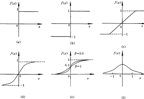
激励函数在预测层，判断哪些值要被送到预测结果那里：

TensorFlow 常用的 activation function

• 添加神经层：

输入参数有 inputs, in_size, out_size, 和 activation_function

import tensorflow as tf

def add_layer(inputs, in_size, out_size,  activation_function=None):

  Weights = tf.Variable(tf.random_normal([in_size, out_size]))
  biases = tf.Variable(tf.zeros([1, out_size]) + 0.1)
  Wx_plus_b = tf.matmul(inputs, Weights) + biases

  if activation_function is None:
    outputs = Wx_plus_b
  else:
    outputs = activation_function(Wx_plus_b)

return outputs

• 分类问题的 loss 函数 cross_entropy ：

# the error between prediction and real data
# loss 函数用 cross entropy
cross_entropy = tf.reduce_mean(-tf.reduce_sum(ys * tf.log(prediction),
                                              reduction_indices=[1]))       # loss
train_step = tf.train.GradientDescentOptimizer(0.5).minimize(cross_entropy)

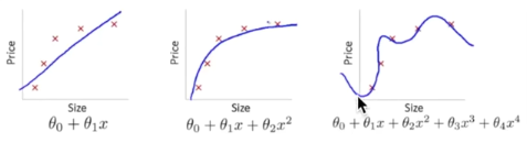
• overfitting：

下面第三个图就是 overfitting，就是过度准确地拟合了历史数据，而对新数据预测时就会有很大误差：

Tensorflow 有一个很好的工具, 叫做dropout, 只需要给予它一个不被 drop 掉的百分比，就能很好地降低 overfitting。

dropout 是指在深度学习网络的训练过程中，按照一定的概率将一部分神经网络单元暂时从网络中丢弃，相当于从原始的网络中找到一个更瘦的网络，这篇博客中讲的非常详细

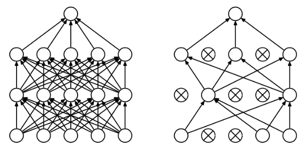
代码实现就是在 add layer 函数里加上 dropout, keep_prob 就是保持多少不被 drop，在迭代时在 sess.run 中被 feed:

def add_layer(inputs, in_size, out_size, layer_name, activation_function=None, ):
    # add one more layer and return the output of this layer
    Weights = tf.Variable(tf.random_normal([in_size, out_size]))
    biases = tf.Variable(tf.zeros([1, out_size]) + 0.1, )
    Wx_plus_b = tf.matmul(inputs, Weights) + biases

    # here to dropout
    # 在 Wx_plus_b 上drop掉一定比例
    # keep_prob 保持多少不被drop，在迭代时在 sess.run 中 feed
    Wx_plus_b = tf.nn.dropout(Wx_plus_b, keep_prob)

    if activation_function is None:
        outputs = Wx_plus_b
    else:
        outputs = activation_function(Wx_plus_b, )
    tf.histogram_summary(layer_name + '/outputs', outputs)  
    return outputs

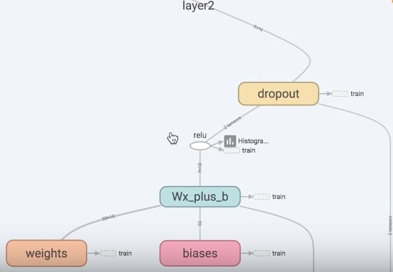
5. 可视化 Tensorboard

Tensorflow 自带 tensorboard ，可以自动显示我们所建造的神经网络流程图：

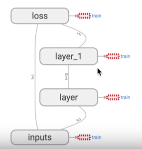
就是用 with tf.name_scope 定义各个框架，注意看代码注释中的区别：

import tensorflow as tf


def add_layer(inputs, in_size, out_size, activation_function=None):
    # add one more layer and return the output of this layer
    # 区别：大框架，定义层 layer，里面有 小部件
    with tf.name_scope('layer'):
        # 区别：小部件
        with tf.name_scope('weights'):
            Weights = tf.Variable(tf.random_normal([in_size, out_size]), name='W')
        with tf.name_scope('biases'):
            biases = tf.Variable(tf.zeros([1, out_size]) + 0.1, name='b')
        with tf.name_scope('Wx_plus_b'):
            Wx_plus_b = tf.add(tf.matmul(inputs, Weights), biases)
        if activation_function is None:
            outputs = Wx_plus_b
        else:
            outputs = activation_function(Wx_plus_b, )
        return outputs


# define placeholder for inputs to network
# 区别：大框架，里面有 inputs x，y
with tf.name_scope('inputs'):
    xs = tf.placeholder(tf.float32, [None, 1], name='x_input')
    ys = tf.placeholder(tf.float32, [None, 1], name='y_input')

# add hidden layer
l1 = add_layer(xs, 1, 10, activation_function=tf.nn.relu)
# add output layer
prediction = add_layer(l1, 10, 1, activation_function=None)

# the error between prediciton and real data
# 区别：定义框架 loss
with tf.name_scope('loss'):
    loss = tf.reduce_mean(tf.reduce_sum(tf.square(ys - prediction),
                                        reduction_indices=[1]))

# 区别：定义框架 train
with tf.name_scope('train'):
    train_step = tf.train.GradientDescentOptimizer(0.1).minimize(loss)

sess = tf.Session()

# 区别：sess.graph 把所有框架加载到一个文件中放到文件夹"logs/"里 
# 接着打开terminal，进入你存放的文件夹地址上一层，运行命令 tensorboard --logdir='logs/'
# 会返回一个地址，然后用浏览器打开这个地址，在 graph 标签栏下打开
writer = tf.train.SummaryWriter("logs/", sess.graph)
# important step
sess.run(tf.initialize_all_variables())

运行完上面代码后，打开 terminal，进入你存放的文件夹地址上一层，运行命令 tensorboard --logdir='logs/' 后会返回一个地址，然后用浏览器打开这个地址，点击 graph 标签栏下就可以看到流程图了：

6. 保存和加载

训练好了一个神经网络后，可以保存起来下次使用时再次加载：

import tensorflow as tf
import numpy as np

## Save to file
# remember to define the same dtype and shape when restore
W = tf.Variable([[1,2,3],[3,4,5]], dtype=tf.float32, name='weights')
b = tf.Variable([[1,2,3]], dtype=tf.float32, name='biases')

init= tf.initialize_all_variables()

saver = tf.train.Saver()

# 用 saver 将所有的 variable 保存到定义的路径
with tf.Session() as sess:
   sess.run(init)
   save_path = saver.save(sess, "my_net/save_net.ckpt")
   print("Save to path: ", save_path)


################################################

# restore variables
# redefine the same shape and same type for your variables
W = tf.Variable(np.arange(6).reshape((2, 3)), dtype=tf.float32, name="weights")
b = tf.Variable(np.arange(3).reshape((1, 3)), dtype=tf.float32, name="biases")

# not need init step

saver = tf.train.Saver()
# 用 saver 从路径中将 save_net.ckpt 保存的 W 和 b restore 进来
with tf.Session() as sess:
    saver.restore(sess, "my_net/save_net.ckpt")
    print("weights:", sess.run(W))
    print("biases:", sess.run(b))

tensorflow 现在只能保存 variables，还不能保存整个神经网络的框架，所以再使用的时候，需要重新定义框架，然后把 variables 放进去学习。

 原文链接：http://www.jianshu.com/p/e112012a4b2d