相关文章:时间序列分析之ARIMA模型预测__SAS篇
之前一直用SAS做ARIMA模型预测,今天尝试用了一下R,发现灵活度更高,结果输出也更直观。现在记录一下如何用R分析ARIMA模型。
1. 处理数据
1.1. 导入forecast包
forecast包是一个封装的ARIMA统计软件包,在默认情况下,R没有预装forecast包,因此需要先安装该包
> install.packages("forecast')
导入依赖包zoo,再导入forecast包
> library("zoo")
> library("forecast")
1.2. 导入数据
博主使用的数据是一组航空公司的销售数据,可在此下载数据:airline.txt,共有132条数据,是以月为单位的销售数据。
> airline <- read.table("airline.txt")
> airline
V1 V2
1 1 112
2 2 118
3 3 132
4 4 129
5 5 121
6 6 135
7 7 148
8 8 148
9 9 136
10 10 119
(........)
1.3. 将数据转化为时间序列格式(ts)
由于将数据转化为时间序列格式,我们并不需要时间字段,因此只取airline数据的第二列,即销售数据,又因为该数据是以月为单位的,因此Period是12。
> airline2 <- ariline[2]
> airts <- ts(airline2,start=1,frequency=12)
2. 识别模型
2.1. 查看趋势图
> plot.ts(airts)

由图可见,该序列还不平稳,先做一次Log平滑,再做一次差分:
> airlog <- log(airts)
> airdiff <- diff(airlog, differences=1)
> plot.ts(airdiff)
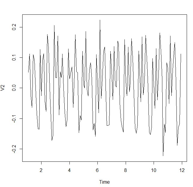
这次看上去就比较平稳了,现在看看ACF和PACF的结果
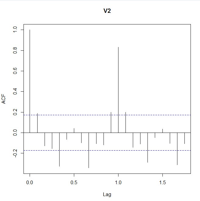
2.2. 查看ACF和PACF
> acf(airdff, lag.max=30)
> acf(airdff, lag.max=30,plot=FALSE)

Autocorrelations of series ‘airdiff’, by lag
0.0000 0.0833 0.1667 0.2500 0.3333 0.4167 0.5000 0.5833 0.6667 0.7500 0.8333
1.000 0.188 -0.127 -0.154 -0.326 -0.066 0.041 -0.098 -0.343 -0.109 -0.120
0.9167 1.0000 1.0833 1.1667 1.2500 1.3333 1.4167 1.5000 1.5833 1.6667 1.7500
0.199 0.833 0.198 -0.143 -0.110 -0.288 -0.046 0.036 -0.104 -0.313 -0.106
1.8333 1.9167 2.0000 2.0833 2.1667 2.2500 2.3333 2.4167 2.5000
-0.085 0.185 0.714 0.175 -0.126 -0.077 -0.214 -0.046 0.029
> pacf(airdff, lag.max=30)
> pacf(airdff, lag.max=30,plot=FALSE)

Partial autocorrelations of series ‘airdiff’, by lag
0.0833 0.1667 0.2500 0.3333 0.4167 0.5000 0.5833 0.6667 0.7500 0.8333 0.9167
0.188 -0.169 -0.101 -0.317 0.018 -0.072 -0.199 -0.509 -0.171 -0.553 -0.300
1.0000 1.0833 1.1667 1.2500 1.3333 1.4167 1.5000 1.5833 1.6667 1.7500 1.8333
0.551 0.010 -0.200 0.164 -0.052 -0.037 -0.108 0.094 0.005 -0.095 -0.001
1.9167 2.0000 2.0833 2.1667 2.2500 2.3333 2.4167 2.5000
0.057 -0.074 -0.048 0.024 0.073 0.047 0.010 0.033
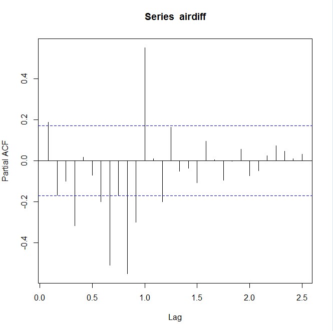
从ACF和PACF可以看出来,该序列在lag=12和lag=24处有明显的spike,说明该序列需要再做一次diff=12的差分。且PACF比ACF呈现更明显的指数平滑的趋势,因此先猜测ARIMA模型为:ARIMA(0,1,1)(0,1,1)[12].
2.3. 利用auto.arima
> auto.arima(airlog,trace=T)

 ARIMA(2,1,2)(1,1,1)[12]                    : -354.4719
 ARIMA(0,1,0)(0,1,0)[12]                    : -316.8213
 ARIMA(1,1,0)(1,1,0)[12]                    : -356.4353
 ARIMA(0,1,1)(0,1,1)[12]                    : -359.7679
 ARIMA(0,1,1)(1,1,1)[12]                    : -354.9069
 ARIMA(0,1,1)(0,1,0)[12]                    : -327.5759
 ARIMA(0,1,1)(0,1,2)[12]                    : -357.6861
 ARIMA(0,1,1)(1,1,2)[12]                    : -363.2418
 ARIMA(1,1,1)(1,1,2)[12]                    : -359.6535
 ARIMA(0,1,0)(1,1,2)[12]                    : -346.1537
 ARIMA(0,1,2)(1,1,2)[12]                    : -361.1765
 ARIMA(1,1,2)(1,1,2)[12]                    : 1e+20
 ARIMA(0,1,1)(1,1,2)[12]                    : -363.2418
 ARIMA(0,1,1)(2,1,2)[12]                    : -368.8244
 ARIMA(0,1,1)(2,1,1)[12]                    : -368.1761
 ARIMA(1,1,1)(2,1,2)[12]                    : -367.0903
 ARIMA(0,1,0)(2,1,2)[12]                    : -363.7024
 ARIMA(0,1,2)(2,1,2)[12]                    : -366.6877
 ARIMA(1,1,2)(2,1,2)[12]                    : 1e+20
 ARIMA(0,1,1)(2,1,2)[12]                    : -368.8244

 Best model: ARIMA(0,1,1)(2,1,2)[12]

Series: airlog
ARIMA(0,1,1)(2,1,2)[12]

Coefficients:
          ma1     sar1     sar2     sma1     sma2
      -0.2710  -0.4764  -0.1066  -0.0098  -0.1987
s.e.   0.0995   0.1432   0.1087   0.1567   0.1130

sigma^2 estimated as 0.001188:  log likelihood=231.88
AIC=-369.57   AICc=-368.82   BIC=-352.9
auto.arima提供的最佳模型为ARIMA(0,1,1)(2,1,2)[12],我们可以同时测试两个模型,看看哪个更适合。
3. 参数估计
> airarima1 <- arima(airlog,order=c(0,1,1),seasonal=list(order=c(0,1,1),period=12),method="ML")
> airarima1
Series: airlog
ARIMA(0,1,1)(0,1,1)[12]

Coefficients:
          ma1     sma1
      -0.3484  -0.5622
s.e.   0.0943   0.0774

sigma^2 estimated as 0.001313:  log likelihood=223.63
AIC=-441.26   AICc=-441.05   BIC=-432.92

> airarima2 <- arima(airlog,order=c(0,1,1),seasonal=list(order=c(2,1,2),period=12),method="ML")
> airarima2
Series: airlog
ARIMA(0,1,1)(2,1,2)[12]

Coefficients:
          ma1    sar1     sar2     sma1    sma2
      -0.3546  1.0614  -0.1211  -1.9130  0.9962
s.e.   0.0995  0.1094   0.1844   0.3887  0.3812

sigma^2 estimated as 0.0009811:  log likelihood=225.56
AIC=-439.12   AICc=-438.37   BIC=-422.44
两个ARIMA模型都采用极大似然方法估计,计算系数对应的t值:
ARIMA(0,1,1)(0,1,1)[12] :t(ma1)=-39.1791, t(sma1)=-93.8445
ARIMA(0,1,1)(2,1,2)[12] : t(ma1)=-35.8173,t(sar1)=88.68383,t(sar2)=-3.56141,t(sma1)=-12.6615,t(sma2)= 6.855526
可见两个模型的系数都是显著的,而ARIMA(0,1,1)(0,1,1)[12]的AIC和BIC比ARIMA(0,1,1)(2,1,2)[12]的要小,因此选择模型ARIMA(0,1,1)(0,1,1)[12]。
4. 预测
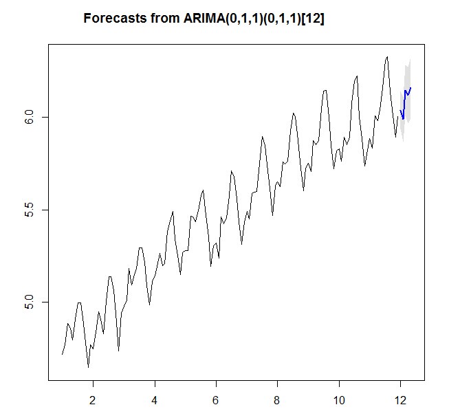
预测五年后航空公司的销售额:
> airforecast <- forecast.Arima(airarima1,h=5,level=c(99.5))
> airforecast
Point Forecast Lo 99.5 Hi 99.5
Jan 12 6.038649 5.936951 6.140348
Feb 12 5.988762 5.867380 6.110143
Mar 12 6.145428 6.007137 6.283719
Apr 12 6.118993 5.965646 6.272340
May 12 6.159657 5.992605 6.326709

> plot.forecast(airforecast)