1. RGB图像灰度化
-
分量法
将彩色图像中的三分量的亮度作为三个灰度图像的灰度值,可根据应用需要选取一种灰度图像。
-
最大值法
将彩色图像中的三分量亮度的最大值作为灰度图的灰度值。
-
平均值法
将彩色图像中的三分量亮度求平均得到一个灰度值。
-
加权平均法
根据重要性及其它指标,将三个分量以不同的权值进行加权平均。由于人眼对绿色的敏感最高,对蓝色敏感最低,因此,按下式对RGB三分量进行加权平均能得到较合理的灰度图像。
2. 二值化
import cv2
import numpy as np

# Read image
img = cv2.imread("imori.jpg").astype(np.float)
b = img[:, :, 0].copy()
g = img[:, :, 1].copy()
r = img[:, :, 2].copy()

# Grayscale
out = 0.2126 * r + 0.7152 * g + 0.0722 * b
out = out.astype(np.uint8)

# Binarization
th = 128
out[out < th] = 0
out[out >= th] = 255

# Save result
cv2.imwrite("out.jpg", out)
cv2.imshow("result", out)
cv2.waitKey(0)
cv2.destroyAllWindows()
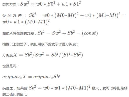
3. OSTU: 大津二值化算法
最大类间方差法是由日本学者大津于1979年提出的,是一种自适应的阈值确定的方法,又叫大津
法,简称OTSU。它是按图像的灰度特性,将图像分成背景和目标2部分。背景和目标之间的类间方差
越大,说明构成图像的2部分的差别越大,当部分目标错分为背景或部分背景错分为目标都会导致2部
分差别变小。因此,使类间方差最大的分割意味着错分概率最小。
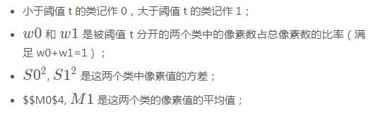
也就是说:
import cv2
import numpy as np

# Read image
img = cv2.imread("imori.jpg").astype(np.float)

H, W, C = img.shape

# Grayscale
out = 0.2126 * img[..., 2] + 0.7152 * img[..., 1] + 0.0722 * img[..., 0]
out = out.astype(np.uint8)

# Determine threshold of Otsu's binarization
max_sigma = 0
max_t = 0

for _t in range(1, 255):
    v0 = out[np.where(out < _t)]
    m0 = np.mean(v0) if len(v0) > 0 else 0.
    w0 = len(v0) / (H * W)
    v1 = out[np.where(out >= _t)]
    m1 = np.mean(v1) if len(v1) > 0 else 0.
    w1 = len(v1) / (H * W)
    sigma = w0 * w1 * ((m0 - m1) ** 2)
    if sigma > max_sigma:
        max_sigma = sigma
        max_t = _t

# Binarization
print("threshold >>", max_t)
th = max_t
out[out < th] = 0
out[out >= th] = 255

# Save result
cv2.imwrite("out.jpg", out)
cv2.imshow("result", out)
cv2.waitKey(0)
cv2.destroyAllWindows()
4. Pooling: 最大池化
# Max Pooling
out = img.copy()

H, W, C = img.shape
G = 8
Nh = int(H / G)
Nw = int(W / G)

for y in range(Nh):
    for x in range(Nw):
        for c in range(C):
            out[G*y:G*(y+1), G*x:G*(x+1), c] = np.max(out[G*y:G*(y+1), G*x:G*(x+1), c])
5. 高斯滤波
高斯滤波器是一种可以使图像平滑的滤波器,用于去除噪声。可用于去除噪声的滤波器还有中值滤波器,平滑滤波器、LoG 滤波器。
高斯滤波器将中心像素周围的像素按照高斯分布加权平均进行平滑化。这样的(二维)权值通常被称为卷积核或者滤波器。
但是,由于图像的长宽可能不是滤波器大小的整数倍,因此我们需要在图像的边缘补0。这种方法称作 Zero Padding。并且权值(卷积核)要进行归一化操作 ( ∑g=1 )。
权值 g(x,y,s) = 1/ (s*sqrt(2 * pi)) * exp( - (x^2 + y^2) / (2*s^2))
标准差 s = 1.3 的 8 近邻 高斯滤波器如下:
             1 2 1
K = 1/16 * [ 2 4 2 ]
             1 2 1
代码实现:
# Gaussian Filter
K_size = 3
sigma = 1.3

## 6. Zero padding
pad = K_size // 2
out = np.zeros((H + pad*2, W + pad*2, C), dtype=np.float)
out[pad:pad+H, pad:pad+W] = img.copy().astype(np.float)

## 7. Kernel
K = np.zeros((K_size, K_size), dtype=np.float)
for x in range(-pad, -pad+K_size):
    for y in range(-pad, -pad+K_size):
        K[y+pad, x+pad] = np.exp( -(x**2 + y**2) / (2* (sigma**2)))

K /= (sigma * np.sqrt(2 * np.pi))
K /= K.sum()

tmp = out.copy()

for y in range(H):
    for x in range(W):
        for c in range(C):
            out[pad+y, pad+x, c] = np.sum(K * tmp[y:y+K_size, x:x+K_size, c])

out = out[pad:pad+H, pad:pad+W].astype(np.uint8)
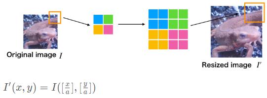
8. 最邻近插值
使用最邻近插值将图像放大1.51.5倍吧!
Opencv最近邻插值在图像放大时补充的像素取最临近的像素的值。由于方法简单,所以处理速度很快,但是放大图像画质劣化明显。
使用下面的公式放大图像吧!I’I’为放大后图像,II为放大前图像,aa为放大率,方括号是四舍五入取整操作:
import cv2
import numpy as np
import matplotlib.pyplot as plt

# Nereset Neighbor interpolation
def nn_interpolate(img, ax=1, ay=1):
    H, W, C = img.shape

    aH = int(ay * H)
    aW = int(ax * W)

    y = np.arange(aH).repeat(aW).reshape(aW, -1)
    x = np.tile(np.arange(aW), (aH, 1))
    y = np.round(y / ay).astype(np.int)
    x = np.round(x / ax).astype(np.int)

    out = img[y,x]
    out = out.astype(np.uint8)
    return out

# Read image
img = cv2.imread("imori.jpg").astype(np.float)

# Nearest Neighbor
out = nn_interpolate(img, ax=1.5, ay=1.5)
9. Canny边缘检测
import cv2
import numpy as np
import matplotlib.pyplot as plt

def Canny_step1(img):
    # Gray scale
    def BGR2GRAY(img):
        ...
    def gaussian_filter(img, K_size=3, sigma=1.3):
        ...
    def sobel_filter(img, K_size=3):
        ...

    def get_edge_angle(fx, fy):
        # get edge strength
        edge = np.sqrt(np.power(fx, 2) + np.power(fy, 2))
        # fx[np.abs(fx) < 1e-5] = 1e-5
        fx = np.maximum(fx, 1e-5)
        angle = np.arctan(fy / fx)
        return edge, angle

    def angle_quantization(angle):
        angle = angle / np.pi * 180
        angle[angle < -22.5] = 180 + angle[angle < -22.5]
        _angle = np.zeros_like(angle, dtype=np.uint8)
        _angle[np.where(angle <= 22.5)] = 0
        _angle[np.where((angle > 22.5) & (angle <= 67.5))] = 45
        _angle[np.where((angle > 67.5) & (angle <= 112.5))] = 90
        _angle[np.where((angle > 112.5) & (angle <= 157.5))] = 135
        return _angle

    gray = BGR2GRAY(img)
    gaussian = gaussian_filter(gray, K_size=5, sigma=1.4)
    fy, fx = sobel_filter(gaussian, K_size=3)
    edge, angle = get_edge_angle(fx, fy)
    angle = angle_quantization(angle)
    return edge, angle

# Read image
img = cv2.imread("imori.jpg").astype(np.float32)

# Canny (step1)
edge, angle = Canny_step1(img)

edge = edge.astype(np.uint8)
angle = angle.astype(np.uint8)

# Save result
cv2.imwrite("out.jpg", edge)
cv2.imshow("result", edge)
cv2.imwrite("out2.jpg", angle)
cv2.imshow("result2", angle)
cv2.waitKey(0)
cv2.destroyAllWindows()
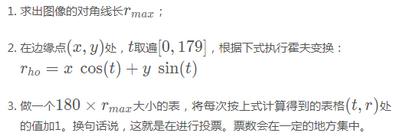
10. Hough Transform: 霍夫变换
霍夫变换,是将座标由直角座标系变换到极座标系,然后再根据数学表达式检测某些形状(如直线和圆)的方法。当直线上的点变换到极座标中的时候,会交于一定的rr、tt的点。这个点即为要检测的直线的参数。通过对这个参数进行逆变换,我们就可以求出直线方程。
方法如下:
- 我们用边缘图像来对边缘像素进行霍夫变换。
- 在霍夫变换后获取值的直方图并选择最大点。
- 对极大点的r和t的值进行霍夫逆变换以获得检测到的直线的参数。
在这里,进行一次霍夫变换之后,可以获得直方图。算法如下:
import cv2
import numpy as np
import matplotlib.pyplot as plt

def Canny(img):
    def BGR2GRAY(img):
        # Gray scale
    def gaussian_filter(img, K_size=3, sigma=1.3):
        # Gaussian filter for grayscale
    def sobel_filter(img, K_size=3):
        # sobel filter
    def get_edge_angle(fx, fy):
        # 同上
    def angle_quantization(angle):
        # 同上
    def non_maximum_suppression(angle, edge):
        H, W = angle.shape
        _edge = edge.copy()

        for y in range(H):
            for x in range(W):
                if angle[y, x] == 0:
                        dx1, dy1, dx2, dy2 = -1, 0, 1, 0
                elif angle[y, x] == 45:
                        dx1, dy1, dx2, dy2 = -1, 1, 1, -1
                elif angle[y, x] == 90:
                        dx1, dy1, dx2, dy2 = 0, -1, 0, 1
                elif angle[y, x] == 135:
                        dx1, dy1, dx2, dy2 = -1, -1, 1, 1
                if x == 0:
                        dx1 = max(dx1, 0)
                        dx2 = max(dx2, 0)
                if x == W-1:
                        dx1 = min(dx1, 0)
                        dx2 = min(dx2, 0)
                if y == 0:
                        dy1 = max(dy1, 0)
                        dy2 = max(dy2, 0)
                if y == H-1:
                        dy1 = min(dy1, 0)
                        dy2 = min(dy2, 0)
                if max(max(edge[y, x], edge[y + dy1, x + dx1]), edge[y + dy2, x + dx2]) != edge[y, x]:
                        _edge[y, x] = 0
        return _edge

    def hysterisis(edge, HT=100, LT=30):
        H, W = edge.shape

        # Histeresis threshold
        edge[edge >= HT] = 255
        edge[edge <= LT] = 0

        _edge = np.zeros((H + 2, W + 2), dtype=np.float32)
        _edge[1 : H + 1, 1 : W + 1] = edge

        ## 8 - Nearest neighbor
        nn = np.array(((1., 1., 1.), (1., 0., 1.), (1., 1., 1.)), dtype=np.float32)

        for y in range(1, H+2):
                for x in range(1, W+2):
                        if _edge[y, x] < LT or _edge[y, x] > HT:
                                continue
                        if np.max(_edge[y-1:y+2, x-1:x+2] * nn) >= HT:
                                _edge[y, x] = 255
                        else:
                                _edge[y, x] = 0

        edge = _edge[1:H+1, 1:W+1]
        return edge

    gray = BGR2GRAY(img)
    gaussian = gaussian_filter(gray, K_size=5, sigma=1.4)
    fy, fx = sobel_filter(gaussian, K_size=3)
    edge, angle = get_edge_angle(fx, fy)
    angle = angle_quantization(angle)
    edge = non_maximum_suppression(angle, edge)
    out = hysterisis(edge, 100, 30)
    return out

def Hough_Line_step1(edge):
    ## Voting
    def voting(edge):
        H, W = edge.shape
        drho = 1
        dtheta = 1
        # get rho max length
        rho_max = np.ceil(np.sqrt(H ** 2 + W ** 2)).astype(np.int)
        # hough table
        hough = np.zeros((rho_max * 2, 180), dtype=np.int)
        # get index of edge
        ind = np.where(edge == 255)
        ## hough transformation
        for y, x in zip(ind[0], ind[1]):
            for theta in range(0, 180, dtheta):
                    # get polar coordinat4s
                    t = np.pi / 180 * theta
                    rho = int(x * np.cos(t) + y * np.sin(t))
                    # vote
                    hough[rho + rho_max, theta] += 1

        out = hough.astype(np.uint8)
        return out

    out = voting(edge)
    return out

# Read image
img = cv2.imread("thorino.jpg").astype(np.float32)
edge = Canny(img)
out = Hough_Line_step1(edge)

out = out.astype(np.uint8)

# Save result
cv2.imwrite("out.jpg", out)
cv2.imshow("result", out)
cv2.waitKey(0)
cv2.destroyAllWindows()