CNN实战2：CIFAR-10数据集上的图像识别

0. 滴不尽相思血泪抛红豆

    上一节讲述了如何通过CNN提取一幅图像的特征后，并将提取的“滤镜”应用于另外一幅图像。其实利用CNN产生这种艺术作品的应用和论文还有很多，例如google著名的DeepDream，它利用以及训练好的网络（例如一个二分类猫狗的网络），识别任意图片（例如一朵云的图片）后将其判别为猫或者狗，并将猫狗的特征复刻到云朵照片上，使计算机“做梦”一样，看到云朵而联想到猫狗，从而创造了新的艺术作品。利用CIFAR-1000训练好的网络来产生DeepDream效果如下图所示：

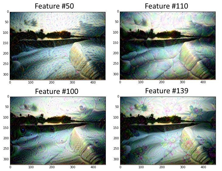
    可以看到，上图中的一些斑点、花纹、水波都是原图中不曾出现的。而通过CIFAR-1000训练的分类网络，在读取图片时，将图片某些局部信息分类为了水波、花纹、斑点等，再通过局部特征信息提取、融合某个分类的特征，从而创作了上述作品。因为这个内容的实际应用不是很大，所以之后的博客看情况再决定要不要贴出来这一块的内容。

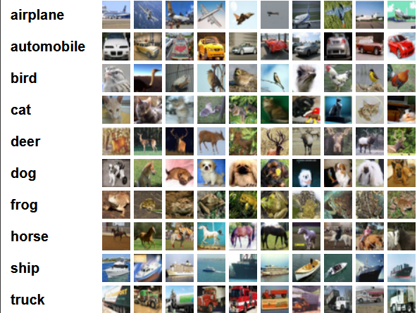
    本篇博客要完成的是更基础的内容。通过CIFAR-10训练集，训练CNN网络来进行图像分类。首先认识一下CIFAR-10训练集。

    CIFAR-10共有60000张32*32像素的图片，被分为10个类别（是不是有点像MNIST呢，但是难度有上升呢），每一类自然有6000张图片。数据集链接为http://www.cs.toronto.edu/~kriz/cifar.html（170.1MB，无需单独下载啦，为了方便小白猫已经把下载写到代码里了，运行python会自动在代码根目录产生temp文件夹存放数据集）。CIFAR-10的分类示例如下图所示：

1. 看不完春柳春花满画楼

  1.1 代码

    在之前章节也提到过，CNN网络中的基本步骤是重复conv-relu-pool后，再加上全连接层后通过softmax输出最后分类概率向量，误差函数由softmax loss构成。其中conv-relu-pool的重复是加深CNN网络的基础方法，它能让网络更复杂准确率更高。所以针对CAFIA-10的图像分类代码和之前的MNIST只是在网络深度上有了差别。

    使用50k图片进行训练，10k图片进行测试。另外值得注意的是，训练集较大时（本例的50k图片）不能全部放入内存。参考tensorflow的官方文档，需要创建一个图像数据读取器，每次训练喂入一个批量的数据，防止内存溢出。相同的，测试时也一批一批的进行测试，计算平均准确率。

    CPU条件下大概要运行1.5-2小时。代码如下：

# CNN Model: CIFAR-10
#---------------------------------------
#
# Author: allen
# Date: 2018.4.20-4.23

import os
import sys
import tarfile
import matplotlib.pyplot as plt
import numpy as np
import tensorflow as tf
from six.moves import urllib
from tensorflow.python.framework import ops
ops.reset_default_graph()

# 目录
abspath = os.path.abspath(__file__)
dname = os.path.dirname(abspath)
os.chdir(dname)

# 开始计算图会话
sess = tf.Session()

# 模型参数
batch_size = 128 # 批量的大小，一次训练和测试的批量大小为128张图片
data_dir = 'temp' # CIFAR-10数据集位置
output_every = 50 # 每训练50次打印一次训练状态
generations = 20000 # 训练20000轮
eval_every = 500 # 每迭代500次，在测试集上进行评估（交叉评估）
image_height = 32
image_width = 32
crop_height = 24
crop_width = 24
num_channels = 3 # 颜色通道（红绿蓝）
num_targets = 10 # 目标分类数
extract_folder = 'cifar-10-batches-bin'

# 初始学习率为0.1，每迭代250次衰减一次学习率。公式为0.1*0.9^(x/250)，x为迭代次数
learning_rate = 0.1
lr_decay = 0.1
num_gens_to_wait = 250.

# 读取二进制CIFA-10图片的参数
image_vec_length = image_height * image_width * num_channels
record_length = 1 + image_vec_length # ( + 1 for the 0-9 label)


# 设置下载CIFA-10图像数据集的URL。下载时在代码目录下创建temp文件夹
data_dir = 'temp'
if not os.path.exists(data_dir):
    os.makedirs(data_dir)
cifar10_url = 'http://www.cs.toronto.edu/~kriz/cifar-10-binary.tar.gz'

# temp创建，下载cifar-10-binary.tar.gz
data_file = os.path.join(data_dir, 'cifar-10-binary.tar.gz')
if os.path.isfile(data_file):
    pass
else:
    # 下载.tar.gz压缩包
    def progress(block_num, block_size, total_size):
        progress_info = [cifar10_url, float(block_num * block_size) / float(total_size) * 100.0]
        print(' Downloading {} - {:.2f}%'.format(*progress_info), end="")
    filepath, _ = urllib.request.urlretrieve(cifar10_url, data_file, progress)
    # 解压
    tarfile.open(filepath, 'r:gz').extractall(data_dir)
   

# 定义图片读取函数，利用tensorflow内置的图像修改函数，返回一个打乱顺序后的数据集
def read_cifar_files(filename_queue, distort_images = True):
    reader = tf.FixedLengthRecordReader(record_bytes=record_length)
    key, record_string = reader.read(filename_queue)
    record_bytes = tf.decode_raw(record_string, tf.uint8)
    image_label = tf.cast(tf.slice(record_bytes, [0], [1]), tf.int32)
 
    # 提取图片
    image_extracted = tf.reshape(tf.slice(record_bytes, [1], [image_vec_length]),
                                 [num_channels, image_height, image_width])
   
    # 图片同一形状
    image_uint8image = tf.transpose(image_extracted, [1, 2, 0])
    reshaped_image = tf.cast(image_uint8image, tf.float32)
   
    # 随机打乱图片
    final_image = tf.image.resize_image_with_crop_or_pad(reshaped_image, crop_width, crop_height)
   
    if distort_images:
        final_image = tf.image.random_flip_left_right(final_image)
        final_image = tf.image.random_brightness(final_image,max_delta=63)
        final_image = tf.image.random_contrast(final_image,lower=0.2, upper=1.8)

    final_image = tf.image.per_image_standardization(final_image)
    return(final_image, image_label)


# 声明批处理管道填充函数
def input_pipeline(batch_size, train_logical=True):
    if train_logical:
        files = [os.path.join(data_dir, extract_folder, 'data_batch_{}.bin'.format(i)) for i in range(1,6)]
    else:
        files = [os.path.join(data_dir, extract_folder, 'test_batch.bin')]
    filename_queue = tf.train.string_input_producer(files)
    image, label = read_cifar_files(filename_queue)
   
    # 设置适合的min_after_dequeue很重要。该参数是设置抽样图片缓存最小值。
    # tensorflow官方推荐设置为(#threads + error margin)*batch_size。
    # 如果设置太大会导致更多的shuffle，从图像队列中shuffle大量的图像数据会消耗更多内存。
   
    min_after_dequeue = 5000
    capacity = min_after_dequeue + 3 * batch_size
    example_batch, label_batch = tf.train.shuffle_batch([image, label],
                                                        batch_size=batch_size,
                                                        capacity=capacity,
                                                        min_after_dequeue=min_after_dequeue)

    return(example_batch, label_batch)

   
# 声明CNN模型。（重点部分）
# 由两个卷积层(conv-relu-maxpool)加上三个全连接层组成。
def cifar_cnn_model(input_images, batch_size, train_logical=True):
    def truncated_normal_var(name, shape, dtype):
        return(tf.get_variable(name=name, shape=shape, dtype=dtype, initializer=tf.truncated_normal_initializer(stddev=0.05)))
    def zero_var(name, shape, dtype):
        return(tf.get_variable(name=name, shape=shape, dtype=dtype, initializer=tf.constant_initializer(0.0)))
   
    # 第一个卷积层（conv-relu-maxpool）
    with tf.variable_scope('conv1') as scope:
        # 卷积窗口大小为5*5，通道数为3（3种颜色），卷积核个数64（输出特征数）
        conv1_kernel = truncated_normal_var(name='conv_kernel1', shape=[5, 5, 3, 64], dtype=tf.float32)
        # We convolve across the image with a stride size of 1
        conv1 = tf.nn.conv2d(input_images, conv1_kernel, [1, 1, 1, 1], padding='SAME')
        # Initialize and add the bias term
        conv1_bias = zero_var(name='conv_bias1', shape=[64], dtype=tf.float32)
        conv1_add_bias = tf.nn.bias_add(conv1, conv1_bias)
        # ReLU element wise
        relu_conv1 = tf.nn.relu(conv1_add_bias)
   
    # Max Pooling
    pool1 = tf.nn.max_pool(relu_conv1, ksize=[1, 3, 3, 1], strides=[1, 2, 2, 1],padding='SAME', name='pool_layer1')
   
    # Local Response Normalization (parameters from paper)
    # paper: http://papers.nips.cc/paper/4824-imagenet-classification-with-deep-convolutional-neural-networks
    norm1 = tf.nn.lrn(pool1, depth_radius=5, bias=2.0, alpha=1e-3, beta=0.75, name='norm1')

    # 第二个卷积层 同第一个卷积层
    with tf.variable_scope('conv2') as scope:
        # Conv kernel is 5x5, across all prior 64 features and we create 64 more features
        conv2_kernel = truncated_normal_var(name='conv_kernel2', shape=[5, 5, 64, 64], dtype=tf.float32)
        # Convolve filter across prior output with stride size of 1
        conv2 = tf.nn.conv2d(norm1, conv2_kernel, [1, 1, 1, 1], padding='SAME')
        # Initialize and add the bias
        conv2_bias = zero_var(name='conv_bias2', shape=[64], dtype=tf.float32)
        conv2_add_bias = tf.nn.bias_add(conv2, conv2_bias)
        # ReLU element wise
        relu_conv2 = tf.nn.relu(conv2_add_bias)
   
    # Max Pooling
    pool2 = tf.nn.max_pool(relu_conv2, ksize=[1, 3, 3, 1], strides=[1, 2, 2, 1], padding='SAME', name='pool_layer2')   
   
     # Local Response Normalization (parameters from paper)
    norm2 = tf.nn.lrn(pool2, depth_radius=5, bias=2.0, alpha=1e-3, beta=0.75, name='norm2')
   
    # Reshape output into a single matrix for multiplication for the fully connected layers
    reshaped_output = tf.reshape(norm2, [batch_size, -1])
    reshaped_dim = reshaped_output.get_shape()[1].value
   
    # 第一个全连接层
    with tf.variable_scope('full1') as scope:
        # 第一个全连接层有384个输出
        full_weight1 = truncated_normal_var(name='full_mult1', shape=[reshaped_dim, 384], dtype=tf.float32)
        full_bias1 = zero_var(name='full_bias1', shape=[384], dtype=tf.float32)
        full_layer1 = tf.nn.relu(tf.add(tf.matmul(reshaped_output, full_weight1), full_bias1))

    # 第二个全连接层
    with tf.variable_scope('full2') as scope:
        # 第二个全连接层有192个输出 即384->192
        full_weight2 = truncated_normal_var(name='full_mult2', shape=[384, 192], dtype=tf.float32)
        full_bias2 = zero_var(name='full_bias2', shape=[192], dtype=tf.float32)
        full_layer2 = tf.nn.relu(tf.add(tf.matmul(full_layer1, full_weight2), full_bias2))

    # 第三个全连接层 -> 输出10个类别
    with tf.variable_scope('full3') as scope:
        # 最后一个全连接层有10个输出 即192->10
        full_weight3 = truncated_normal_var(name='full_mult3', shape=[192, num_targets], dtype=tf.float32)
        full_bias3 =  zero_var(name='full_bias3', shape=[num_targets], dtype=tf.float32)
        final_output = tf.add(tf.matmul(full_layer2, full_weight3), full_bias3)
       
    return(final_output)


# 损失函数
# 本例使用softmax loss（详见softmax loss节的讲解）
def cifar_loss(logits, targets):
    targets = tf.squeeze(tf.cast(targets, tf.int32))
    cross_entropy = tf.nn.sparse_softmax_cross_entropy_with_logits(logits=logits, labels=targets)
    # 将每个批量测试集准确率均值
    cross_entropy_mean = tf.reduce_mean(cross_entropy, name='cross_entropy')
    return(cross_entropy_mean)


# 定义训练步骤函数
def train_step(loss_value, generation_num):
    # 学习率函数定义（前面已经提到过）
    model_learning_rate = tf.train.exponential_decay(learning_rate, generation_num,
                                                     num_gens_to_wait, lr_decay, staircase=True)
    my_optimizer = tf.train.GradientDescentOptimizer(model_learning_rate)
    # 初始化训练步骤
    train_step = my_optimizer.minimize(loss_value)
    return(train_step)


# 定义准确率函数
# 训练（打乱顺序的）和测试集都可以使用该函数
# 该函数输入logits和目标向量（最后的10个输出），输出平均准确度
def accuracy_of_batch(logits, targets):
    targets = tf.squeeze(tf.cast(targets, tf.int32))
    batch_predictions = tf.cast(tf.argmax(logits, 1), tf.int32)
    predicted_correctly = tf.equal(batch_predictions, targets)
    accuracy = tf.reduce_mean(tf.cast(predicted_correctly, tf.float32))
    return(accuracy)

# Get data
print('Getting/Transforming Data.')
# 初始化训练图像管道和测试图像管道
images, targets = input_pipeline(batch_size, train_logical=True)
test_images, test_targets = input_pipeline(batch_size, train_logical=False)

# 初始化训练模型
print('Creating the CIFAR10 Model.')
with tf.variable_scope('model_definition') as scope:
    model_output = cifar_cnn_model(images, batch_size)
    # 创建训练时需要声明scope.reuse_variables
    # 这样可以在创建测试模型时重用训练模型相同的模型参数
    scope.reuse_variables()
    test_output = cifar_cnn_model(test_images, batch_size)

# 初始化损失函数
print('Declare Loss Function.')
loss = cifar_loss(model_output, targets)

# 准确度函数
accuracy = accuracy_of_batch(test_output, test_targets)

# Create training operations
print('Creating the Training Operation.')
generation_num = tf.Variable(0, trainable=False)
train_op = train_step(loss, generation_num)

# Initialize Variables
print('Initializing the Variables.')
init = tf.global_variables_initializer()
sess.run(init)

# Initialize queue (This queue will feed into the model, so no placeholders necessary)
tf.train.start_queue_runners(sess=sess)

# 开始训练
print('Starting Training')
train_loss = []
test_accuracy = []
for i in range(generations):
    _, loss_value = sess.run([train_op, loss])
   
    if (i+1) % output_every == 0:
        train_loss.append(loss_value)
        output = 'Generation {}: Loss = {:.5f}'.format((i+1), loss_value)
        print(output)
   
    if (i+1) % eval_every == 0:
        [temp_accuracy] = sess.run([accuracy])
        test_accuracy.append(temp_accuracy)
        acc_output = ' --- Test Accuracy = {:.2f}%.'.format(100.*temp_accuracy)
        print(acc_output)

# 打印并绘制损失函数和准确度函数
eval_indices = range(0, generations, eval_every)
output_indices = range(0, generations, output_every)

# 绘制loss曲线
plt.plot(output_indices, train_loss, 'k-')
plt.title('Softmax Loss per Generation')
plt.xlabel('Generation')
plt.ylabel('Softmax Loss')
plt.show()

# 绘制准确度曲线
plt.plot(eval_indices, test_accuracy, 'k-')
plt.title('Test Accuracy')
plt.xlabel('Generation')
plt.ylabel('Accuracy')
plt.show()

  1.2 运行结果

    交互栏的输出，每50轮打印一次loss函数，每500轮打印一次准确率。最终达到了76.56%的分类准确率：

    loss函数和准确率函数变化如下图：

    

    对该实验结果进行一些简单的分析。可以看到loss函数已经比较低了，但是准确度依然不是特别理想。初步归纳的原因有：

• 训练集和测试集较大，训练轮数不够
• 如准确度变化图所示，在20000轮之前有更高的准确度，远优于最终的76%。可能76%的结果陷入了一个局部最优，所以导致loss函数虽然很低但准确度依然不高

    综上分析。如果要进一步优化准确率结果，有以下解决方案：

• 可以考虑加深网络深度，提取更多特征从而提高准确性
• 增加训练轮数，寻找更贴近全局最优的解
• 可以人为对参数进行调优避免局部最优的情况

2. 睡不稳纱窗风雨黄昏后

    本篇博客更新时间较长，代码比之前的要复杂一些，它是一个传统的基于CNN图像分类网络。难度上它比MNIST手写识别网络更深，更难一些；创新性上比不上模仿大师。如果是公路裂痕识别的话，就不应该用分类的思想解决了。而是利用CNN网络将图片与标注（哪些地方是裂痕）作为输入对进行训练。当然，这也跟数据集裂痕图片的label是怎么标注的有关系。

    更完这一篇，如果不更新前文提到的DeepDream的话可能要停止一段时间了，因为小白喵需要一些时间来熟悉这些内容。我看到她坐在前面认真学习着，这就行了。