信用卡欺诈检测Credit Card Fraud Detection(kaggle)

地址：https://www.kaggle.com/mlg-ulb/creditcardfraud

数据概述

数据集包含2013年9月欧洲持卡人通过信用卡进行的交易。
该数据集显示了两天内发生的交易，在284,807笔交易中，我们有492起欺诈。数据集高度不平衡，阳性类别（欺诈）占所有交易的0.172％。

它仅包含数字输入变量，它们是PCA转换的结果。遗憾的是，由于机密性问题，我们无法提供有关数据的原始功能和更多背景信息。功能部件V1，V2，…，V28是使用PCA获得的主要组件，唯一尚未使用PCA转换的功能部件是“时间”和“量”。功能“时间”包含数据集中每个事务和第一个事务之间经过的秒数。功能“金额”是交易金额，此功能可用于与示例相关的成本敏感型学习。要素“类别”是响应变量，在发生欺诈时其值为1，否则为0。

识别欺诈性的信用卡交易。

给定类别不平衡率，我们建议使用精确召回曲线下的面积（AUPRC）测量精度。混淆矩阵的准确性对于不平衡分类没有意义。

还有很多的至于要使用PRC曲线，我们后面在补上，现在先补充代码

这个是使用逻辑回归计算的代码

# -*- coding: utf-8 -*-
"""
Created on Thu Feb 18 17:22:54 2021

@author: Administrator
"""

#%%导入模块
import pandas as pd 
import numpy as np
from scipy import stats
import seaborn as sns
import matplotlib.pyplot as plt
%matplotlib inline
plt.rc("font",family="SimHei",size="12")  #解决中文无法显示的问题


#%%导入数据
creditcard = pd.read_csv('D:/信用卡欺诈检测/creditcard.csv/creditcard.csv')
creditcard.info()
creditcard.isnull().sum()
creditcard.corr().to_excel('tmp1.xlsx')


#%%使用常规的方法
creditcard.Class.mean()  #creditcard.Class,这个属于极度倾斜了  28w条数据



#%%数值变量的iv值计算
num_col = list(creditcard.columns)[1:-1]
num_iv_woedf = pc.WoeDf()
clf = pc.NumBin()
for i in num_col:
    clf.fit(creditcard[i] ,creditcard.Class)
    #clf.generate_transform_fun()
    num_iv_woedf.append(clf.woe_df_)
num_iv_woedf.to_excel('tmp2')

  
# 去掉这些V13    V15    V22    V24    V25    V26
num_col = [i for i in num_col if i not in ['V13',    'V15',    'V22',    'V24',    'V25',    'V26']]
num_iv_woedf = pc.WoeDf()
clf = pc.NumBin()
for i in num_col:
    clf.fit(creditcard[i] ,creditcard.Class)
    creditcard[i+'_bin'] = clf.transform(creditcard[i])  #这样可以省略掉后面转换成_bin的一步骤
    num_iv_woedf.append(clf.woe_df_)


#%%woe转换
bin_col = [i for i in list(creditcard.columns) if i[-4:]=='_bin']

cate_iv_woedf = pc.WoeDf()
for i in bin_col:
    cate_iv_woedf.append(pc.cross_woe(creditcard[i] ,creditcard.Class))
cate_iv_woedf.to_excel('tmp1')
cate_iv_woedf.bin2woe(creditcard,bin_col)


#%%建模
model_col = [i for i in list(creditcard.columns) if i[-4:]=='_woe']

import pandas as pd
import matplotlib.pyplot as plt #导入图像库
import matplotlib
import seaborn as sns
import statsmodels.api as sm
from sklearn.metrics import roc_curve, auc
from sklearn.model_selection import train_test_split

X = creditcard[model_col]
Y = creditcard['Class']


x_train,x_test,y_train,y_test=train_test_split(X,Y,test_size=0.3,random_state=100)


X1=sm.add_constant(x_train)   #在X前加上一列常数1，方便做带截距项的回归
logit=sm.Logit(y_train.astype(float),X1.astype(float))
result=logit.fit()
result.summary()
result.params

resu_1 = result.predict(X1.astype(float))
fpr, tpr, threshold = roc_curve(y_train, resu_1)
rocauc = auc(fpr, tpr)  #0.9693313248601317
plt.plot(fpr, tpr, 'b', label='AUC = %0.2f' % rocauc)
plt.legend(loc='lower right')
plt.plot([0, 1], [0, 1], 'r--')
plt.xlim([0, 1])
plt.ylim([0, 1])
plt.ylabel('真正率')
plt.xlabel('假正率')
plt.show()

# 此处我们看一下混淆矩阵
from sklearn.metrics import precision_score, recall_score, f1_score,confusion_matrix
#lr = LogisticRegression(C=best_c, penalty='l1')
#lr.fit(X_train_undersample, y_train_undersample)
#y_pred_undersample = lr.predict(X_train_undersample)

resu_1 = resu_1.apply(lambda x :1 if x>=0.5 else 0)
matrix = confusion_matrix(y_train, resu_1)
print("混淆矩阵:
", matrix)
print("精度:", precision_score(y_train, resu_1))
print("召回率:", recall_score(y_train, resu_1))
print("f1分数:", f1_score(y_train, resu_1))
'''
混淆矩阵:
 [[198985     29]
 [    73    277]]
精度: 0.9052287581699346
召回率: 0.7914285714285715
f1分数: 0.8445121951219513
'''


#%%验证集
X3 = sm.add_constant(x_test)
resu = result.predict(X3.astype(float))
fpr, tpr, threshold = roc_curve(y_test, resu)
rocauc = auc(fpr, tpr)
plt.plot(fpr, tpr, 'b', label='AUC = %0.2f' % rocauc)
plt.legend(loc='lower right')
plt.plot([0, 1], [0, 1], 'r--')
plt.xlim([0, 1])
plt.ylim([0, 1])
plt.ylabel('真正率')
plt.xlabel('假正率')
plt.show()

# 此处我们看一下混淆矩阵
from sklearn.metrics import precision_score, recall_score, f1_score,confusion_matrix
#lr = LogisticRegression(C=best_c, penalty='l1')
#lr.fit(X_train_undersample, y_train_undersample)
#y_pred_undersample = lr.predict(X_train_undersample)

resu = resu.apply(lambda x :1 if x>=0.5 else 0)
matrix = confusion_matrix(y_test, resu)
print("混淆矩阵:
", matrix)
print("精度:", precision_score(y_test, resu))
print("召回率:", recall_score(y_test, resu))
print("f1分数:", f1_score(y_test, resu))
'''
混淆矩阵:
 [[85275    26]
 [   40   102]]
精度: 0.796875
召回率: 0.7183098591549296
f1分数: 0.7555555555555555
'''







#%%试一下那个度量工具
def tpr_weight_funtion(y_true,y_predict):
    d = pd.DataFrame()
    d['prob'] = list(y_predict)
    d['y'] = list(y_true)
    d = d.sort_values(['prob'], ascending=[0])
    y = d.y
    PosAll = pd.Series(y).value_counts()[1]
    NegAll = pd.Series(y).value_counts()[0]
    pCumsum = d['y'].cumsum()
    nCumsum = np.arange(len(y)) - pCumsum + 1
    pCumsumPer = pCumsum / PosAll
    nCumsumPer = nCumsum / NegAll
    TR1 = pCumsumPer[abs(nCumsumPer-0.001).idxmin()]
    TR2 = pCumsumPer[abs(nCumsumPer-0.005).idxmin()]
    TR3 = pCumsumPer[abs(nCumsumPer-0.01).idxmin()]
    return 0.4 * TR1 + 0.3 * TR2 + 0.3 * TR3

tpr_weight_funtion(y_train, resu_1) #0.8754285714285714

 下面补上xgboost模型的代码

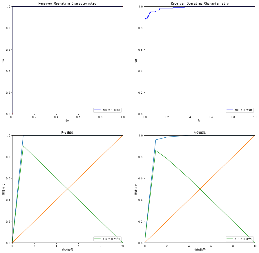
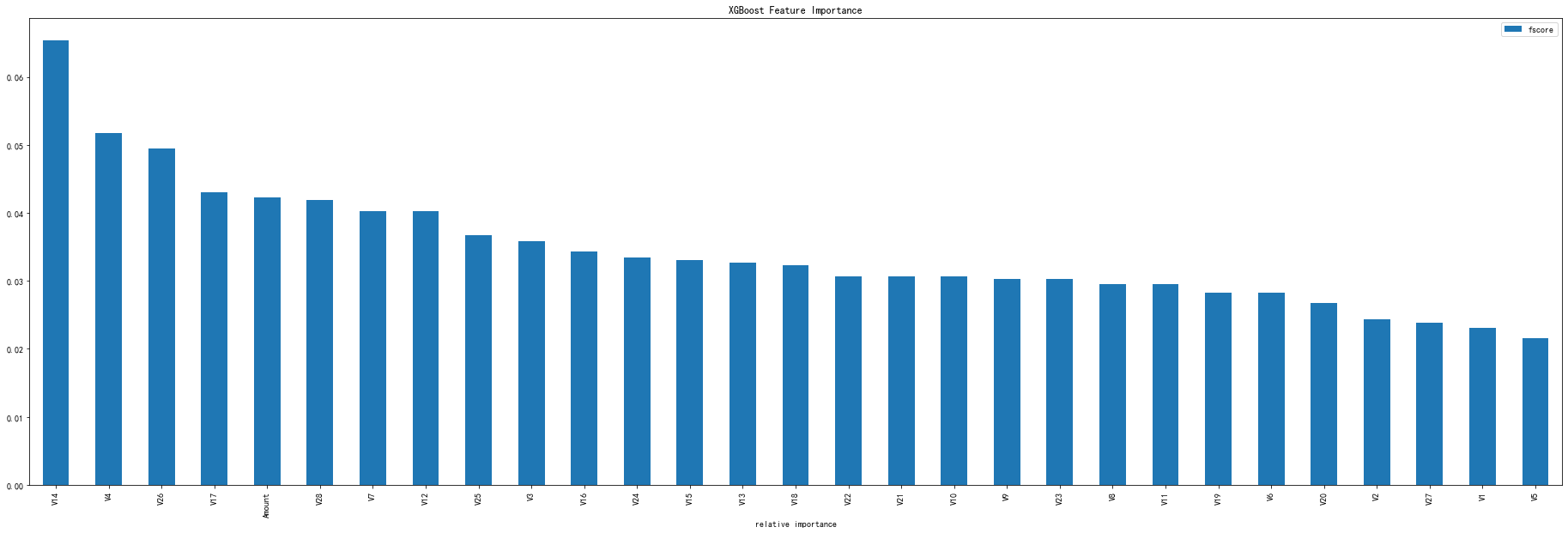
# -*- coding: utf-8 -*-
"""
Created on Wed Mar 10 19:47:40 2021

@author: Administrator
"""


#%%
import numpy as np
import pandas as pd
import matplotlib.pyplot as plt
import operator
import time
import xgboost as xgb
from xgboost import plot_importance  #画特征重要性的函数
#from imblearn.ensemble import EasyEnsemble  #还有模块木有安装
from sklearn.model_selection import train_test_split
#from sklearn.externals import joblib 已经改成了下面这种方式
import joblib
from sklearn.metrics import auc,roc_curve  #说明是分类
plt.rc('font',family='SimHei',size=13)   #使画出的图形中能正常显示中文
%matplotlib inline


#%%导入数据
creditcard = pd.read_csv('D:/信用卡欺诈检测/creditcard.csv/creditcard.csv')


#%%
train_y = creditcard[['Class']]
train_y.columns = ['y']
train_x = creditcard.drop(['Class','Time'],axis=1)


# 
file_xgboost_model='./xgboost_model' #模型文件
file_xgboost_columns='./columns.csv' #最终使用的特征
file_xgboost_model_auc_ks='./xgboost_model_auc_ks.png' #模型AUC和KS值
file_xgboost_model_score='./xgboost_model_score.png' # 模型预测用户的评分分布
file_xgboost_model_prob='./xgboost_model_prob.png' #模型预测用户的概率分布


#%%
def create_feature_map(features):
    outfile = open('xgb.txt', 'w')  #写，新建一个叫xgb.txt的文件
    i = 0
    for feat in features:
        outfile.write('{0}	{1}	q
'.format(i, feat))   #格式为 0  feature  q  	是分隔符，为空  就是说第一列是序号，第二列是特征名称，第三列是q,不知道需要这个q干吗，可以是多写了，先要着吧，后面再看看吧
        i = i + 1
    outfile.close()
create_feature_map(train_x.columns)

#%%
#运行XGBoost,输出特征重要性排名
#运行XGBoost,输出特征重要性排名
def run_xgboost(data_x,data_y,random_state_num):
    train_x,valid_x,train_y,valid_y = train_test_split(data_x.values,data_y.values,test_size=0.25,random_state=random_state_num)
    print('开始训练模型')
    start = time.time()
    #转换成xgb运算格式
    d_train = xgb.DMatrix(train_x,train_y)
    d_valid = xgb.DMatrix(valid_x,valid_y)
    watchlist = [(d_train,'train'),(d_valid,'valid')]
    #参数设置（未调箱前的参数）
    params={
        'eta':0.2,                        #特征权重，取值范围0~1，通常最后设置eta为0.01~0.2
        'max_depth':3,                    #树的深度，通常取值3-10，过大容易过拟合，过小欠拟合
        'min_child_weight':1,             #最小样本的权重，调大参数可以繁殖过拟合
        'gamma':0.4,                      #控制是否后剪枝，越大越保守，一般0.1、 0.2的样子
        'subsample':0.8,                  #随机取样比例
        'colsample_bytree':0.8 ,          #默认为1，取值0~1，对特征随机采集比例
        'reg_lambda':0.8,
        'reg_alpha':0.6,
        'learning_rate':0.1,
        'n_estimators':500,
        'booster':'gbtree',               #迭代树
        'objective':'binary:logistic',    #逻辑回归，输出为概率
        'nthread':6,                      #设置最大的进程量，若不设置则会使用全部资源
        'scale_pos_weight':1,             #默认为0,1可以处理类别不平衡
        'lambda':1,                       #默认为1，用于L2平滑处理项，避免模型过拟合
        'seed':1234,                      #随机树种子
        'silent':1,                       #0表示输出结果
        'eval_metric':'auc'               #评分指标
    }
    bst = xgb.train(params, d_train,1000,watchlist,early_stopping_rounds=100, verbose_eval=5)   #最大迭代次数1000次
    print(time.time()-start)
    tree_nums = bst.best_ntree_limit
    print('最优模型树的数量：%s,最优迭代次数：%s,auc: %s' %(bst.best_ntree_limit,bst.best_iteration,bst.best_score))
    bst = xgb.train(params, d_train,tree_nums,watchlist,early_stopping_rounds=100, verbose_eval=10) #最优模型迭代次数去训练
    
#     feat_imp = pd.Series(clf.booster().get_fscore()).sort_values(ascending=False)
#     #新版需要转换成dict or list 
#     #feat_imp = pd.Series(dict(clf.get_booster().get_fscore())).sort_values(ascending=False)
#     #plt.bar(feat_imp.index, feat_imp)
#     feat_imp.plot(kind='bar', title='Feature Importances')
    #展示特征重要性排名
    feat_imp = bst.get_fscore(fmap='xgb.txt')
    feat_imp = sorted(feat_imp.items(),key=operator.itemgetter(1))
    df = pd.DataFrame(feat_imp,columns=['feature','fscore'])
    #每个特征被调用的次数/所有特征被调用总次数
    df['fscore'] = df['fscore']/df['fscore'].sum()
    #分数高的排在前面,展示前40个重要特征排名
    df = df.sort_values(by='fscore',ascending=False)
    df = df.iloc[:40]
    plt.figure()
    df.plot(kind='bar',x='feature',y='fscore',legend=True,figsize=(32,10))
    plt.title('XGBoost Feature Importance')
    plt.xlabel('relative importance')
    plt.gcf().savefig('feature_importance_xgb.png')
    plt.show()
    return bst

#%%
# 绘制ROC曲线函数
def plot_roc(test_x, test_y):
    predictions = bst.predict(xgb.DMatrix(test_x))
    false_positive_rate, true_positive_rate, thresholds = roc_curve(test_y, predictions)  #roc的几个参数
    roc_auc = auc(false_positive_rate, true_positive_rate)  #直接计算auc
    plt.title('Receiver Operating Characteristic')
    plt.plot(false_positive_rate,true_positive_rate, 'b', label='AUC = %0.4f' % roc_auc)
    plt.legend(loc='lower right')
    plt.plot([0, 1], [0, 1], 'r.')
    plt.xlim([0.0, 1.0])
    plt.ylim([0.0, 1.0])
    plt.ylabel('tpr')
    plt.xlabel('fpr')

# 绘制K-S函数 从大到小排序，分10等分
def plot_ks(test_x, test_y):
    predictions = bst.predict(xgb.DMatrix(test_x))
    false_positive_rate, true_positive_rate, thresholds = roc_curve(test_y, predictions, drop_intermediate=False)
    pre = sorted(predictions, reverse=True)  #reverse参数为True意味着按照降序排序，这是画ks时要求的
    num = []
    for i in range(10):
        num.append((i) * int(len(pre) / 10))
    num.append(len(pre) - 1)
    df = pd.DataFrame()
    df['false_positive_rate'] = false_positive_rate
    df['true_positive_rate'] = true_positive_rate
    df['thresholds'] = thresholds
    data_ks = []
    for i in num:
        data_ks.append(list(df[df['thresholds'] == pre[i]].values[0]))
    data_ks = pd.DataFrame(data_ks)
    data_ks.columns = ['fpr', 'tpr', 'thresholds']
    ks = max(data_ks['tpr'] - data_ks['fpr'])
    plt.title('K-S曲线')
    plt.plot(np.array(range(len(num))), data_ks['tpr'])
    plt.plot(np.array(range(len(num))), data_ks['fpr'])
    plt.plot(np.array(range(len(num))), data_ks['tpr'] - data_ks['fpr'], label='K-S = %0.4f' % ks)
    plt.legend(loc='lower right')
    plt.xlim([0, 10])
    plt.ylim([0.0, 1.0])
    plt.ylabel('累计占比')
    plt.xlabel('分组编号')

# 绘制一张图，包含训练和测试集的ROC、AUC、K-S图形指标。
def auc_ks(train_x, test_x, train_y, test_y):
    plt.figure(figsize=(15, 15))
    plt.subplot(221)
    plot_roc(train_x, train_y)
    plt.subplot(222)
    plot_roc(test_x, test_y)
    plt.subplot(223)
    plot_ks(train_x, train_y)
    plt.subplot(224)
    plot_ks(test_x, test_y)
    plt.savefig(file_xgboost_model_auc_ks)
    plt.show()

#%%
#保存模型、评价指标、选择变量到D盘
def run_main(data_x,data_y):
    global bst
    start=time.time()
    bst=run_xgboost(data_x,data_y,random_state_num=1234)  #为什么要是1234，因为调参时候就是=1234
    joblib.dump(bst, file_xgboost_model)  #joblib的用法https://www.cnblogs.com/wzdLY/p/9630671.html 将模型保存
    print('模型已成功保存在 %s'%(file_xgboost_model))
    train_x, test_x, train_y, test_y = train_test_split(data_x.values, data_y.values, test_size=0.25, random_state=1234)
    auc_ks(train_x, test_x, train_y, test_y)
    print('模型评价指标已保存在：%s'%(file_xgboost_model_auc_ks))
    print('运行共花费时间：%s'%(time.time()-start))
    resu = bst.predict(xgb.DMatrix(test_x))
    

    

if __name__=='__main__':
    run_main(train_x, train_y)
    
#%%单独跑这段，就可以得到混淆矩阵
from sklearn.metrics import precision_score, recall_score, f1_score,confusion_matrix
#lr = LogisticRegression(C=best_c, penalty='l1')
#lr.fit(X_train_undersample, y_train_undersample)
#y_pred_undersample = lr.predict(X_train_undersample)

bst=run_xgboost(train_x, train_y,random_state_num=1234) 
train_x, test_x, train_y, test_y = train_test_split(train_x.values, train_y.values, test_size=0.25, random_state=1234)
resu = bst.predict(xgb.DMatrix(test_x))
resu = pd.DataFrame(resu)
resu.columns=['y']
resu = resu['y'].apply(lambda x:1 if x>0.5 else 0)
resu = resu.values

matrix = confusion_matrix(test_y, resu)
print("混淆矩阵:
", matrix)
print("精度:", precision_score(test_y, resu))
print("召回率:", recall_score(test_y, resu))
print("f1分数:", f1_score(test_y, resu))
'''
混淆矩阵:
 [[71078     6]
 [   32    86]]
精度: 0.9347826086956522
召回率: 0.7288135593220338
f1分数: 0.819047619047619
'''

 

混淆矩阵:
[[71078 6]
[ 32 86]]
精度: 0.9347826086956522
召回率: 0.7288135593220338
f1分数: 0.819047619047619

我们可以看出，xgboost模型还是比逻辑回归模型要好 ，而且我还没有经过调参

 2021.03.12补充LightGBM 

代码如下：

# -*- coding: utf-8 -*-
"""
Created on Fri Mar 12 14:43:16 2021

@author: Administrator
"""

#%%导入模块
import pandas as pd 
import numpy as np
from scipy import stats
import seaborn as sns
import matplotlib.pyplot as plt
%matplotlib inline
plt.rc("font",family="SimHei",size="12")  #解决中文无法显示的问题


#%%导入数据
creditcard = pd.read_csv('D:/信用卡欺诈检测/creditcard.csv/creditcard.csv')
creditcard.info()  #284806
creditcard.isnull().sum()
creditcard.head(3)
creditcard.rename(columns={'Class':'y'},inplace = True)

from sklearn.model_selection import KFold
# 分离数据集，方便进行交叉验证
X_train = creditcard.iloc[:,0:-1]
y_train = creditcard.y

# 5折交叉验证
folds = 5
seed = 2021
kf = KFold(n_splits=folds, shuffle=True, random_state=seed)


#%%对训练集数据进行划分，分成训练集和验证集，并进行相应的操作
from sklearn.model_selection import train_test_split
import lightgbm as lgb
# 数据集划分
X_train_split, X_val, y_train_split, y_val = train_test_split(X_train, y_train, test_size=0.3,stratify=y_train)
train_matrix = lgb.Dataset(X_train_split, label=y_train_split)
valid_matrix = lgb.Dataset(X_val, label=y_val)

params = {
            'boosting_type': 'gbdt',
            'objective': 'binary',
            'learning_rate': 0.1,
            'metric': 'auc',
            'min_child_weight': 1,
            'num_leaves': 10,
            'max_depth': 7,
            'reg_lambda': 0,
            'reg_alpha': 0,
            'feature_fraction': 1,
            'bagging_fraction': 1,
            'bagging_freq': 0,
            'seed': 2020,
            'nthread': 8,
            'silent': True,
            'verbose': -1,
}

"""使用训练集数据进行模型训练"""
model = lgb.train(params, train_set=train_matrix, valid_sets=valid_matrix, 
                  num_boost_round=20000, verbose_eval=1000, early_stopping_rounds=200)
#[847]    valid_0's auc: 0.94372
    
from sklearn import metrics
from sklearn.metrics import roc_auc_score

"""预测并计算roc的相关指标"""
val_pre_lgb = model.predict(X_val, num_iteration=model.best_iteration)
fpr, tpr, threshold = metrics.roc_curve(y_val, val_pre_lgb)
roc_auc = metrics.auc(fpr, tpr)
print('未调参前lightgbm单模型在验证集上的AUC：{}'.format(roc_auc))
"""画出roc曲线图"""
plt.figure(figsize=(8, 8))
plt.title('Validation ROC')
plt.plot(fpr, tpr, 'b', label = 'Val AUC = %0.4f' % roc_auc)
plt.ylim(0,1)
plt.xlim(0,1)
plt.legend(loc='best')
plt.title('ROC')
plt.ylabel('True Positive Rate')
plt.xlabel('False Positive Rate')
# 画出对角线
plt.plot([0,1],[0,1],'r--')
plt.show()


import lightgbm as lgb
"""使用lightgbm 5折交叉验证进行建模预测"""
cv_scores = []
for i, (train_index, valid_index) in enumerate(kf.split(X_train, y_train)):
    print('************************************ {} ************************************'.format(str(i+1)))
    X_train_split, y_train_split, X_val, y_val = X_train.iloc[train_index], y_train[train_index], X_train.iloc[valid_index], y_train[valid_index]
    
    train_matrix = lgb.Dataset(X_train_split, label=y_train_split)
    valid_matrix = lgb.Dataset(X_val, label=y_val)

    params = {
                'boosting_type': 'gbdt',
                'objective': 'binary',
                'learning_rate': 0.1,
                'metric': 'auc',
        
                'min_child_weight': 1e-3,
                'num_leaves': 10,
                'max_depth': -1,
                'reg_lambda': 0,
                'reg_alpha': 0,
                'feature_fraction': 1,
                'bagging_fraction': 1,
                'bagging_freq': 0,
                'seed': 2021,
                'nthread': 8,
                'silent': True,
                'verbose': -1,
    }
    
    model = lgb.train(params, train_set=train_matrix, num_boost_round=20000, valid_sets=valid_matrix, verbose_eval=1000, early_stopping_rounds=200)
    val_pred = model.predict(X_val, num_iteration=model.best_iteration)
    
    cv_scores.append(roc_auc_score(y_val, val_pred))
    print(cv_scores)

print("lgb_scotrainre_list:{}".format(cv_scores))
print("lgb_score_mean:{}".format(np.mean(cv_scores)))
print("lgb_score_std:{}".format(np.std(cv_scores)))


#%%贝叶斯调参
from sklearn.model_selection import cross_val_score

"""定义优化函数"""
def rf_cv_lgb(num_leaves, max_depth, bagging_fraction, feature_fraction, bagging_freq, min_data_in_leaf, 
              min_child_weight, min_split_gain, reg_lambda, reg_alpha):
    # 建立模型
    model_lgb = lgb.LGBMClassifier(boosting_type='gbdt', bjective='binary', metric='auc',
                                   learning_rate=0.1, n_estimators=5000,
                                   num_leaves=int(num_leaves), max_depth=int(max_depth), 
                                   bagging_fraction=round(bagging_fraction, 2), feature_fraction=round(feature_fraction, 2),
                                   bagging_freq=int(bagging_freq), min_data_in_leaf=int(min_data_in_leaf),
                                   min_child_weight=min_child_weight, min_split_gain=min_split_gain,
                                   reg_lambda=reg_lambda, reg_alpha=reg_alpha,
                                   n_jobs= 8
                                  )
    
    val = cross_val_score(model_lgb, X_train_split, y_train_split, cv=5, scoring='roc_auc').mean()
    
    return val

from bayes_opt import BayesianOptimization
"""定义优化参数"""
bayes_lgb = BayesianOptimization(
    rf_cv_lgb, 
    {
        'num_leaves':(10, 200),
        'max_depth':(3, 20),
        'bagging_fraction':(0.5, 1.0),
        'feature_fraction':(0.5, 1.0),
        'bagging_freq':(0, 100),
        'min_data_in_leaf':(10,100),
        'min_child_weight':(0, 10),
        'min_split_gain':(0.0, 1.0),
        'reg_alpha':(0.0, 10),
        'reg_lambda':(0.0, 10),
    }
)

"""开始优化"""
bayes_lgb.maximize(n_iter=10)

bayes_lgb.max
'''
{'target': 0.978984093218777,
 'params': {'bagging_fraction': 0.7852426281123215,
  'bagging_freq': 42.927767267031435,
  'feature_fraction': 0.8729234124911952,
  'max_depth': 18.80072510809031,
  'min_child_weight': 8.29481722055312,
  'min_data_in_leaf': 13.261838180182071,
  'min_split_gain': 0.45972976507462127,
  'num_leaves': 154.4793280962274,
  'reg_alpha': 7.018060276190158,
  'reg_lambda': 2.1475557765094413}}
'''
#%%调整一个较小的学习率，并通过cv函数确定当前最优的迭代次数"""
base_params_lgb = {
                    'boosting_type': 'gbdt',
                    'objective': 'binary',
                    'metric': 'auc',
                    'learning_rate': 0.01,
                    'num_leaves': 154,
                    'max_depth': 18,
                    'min_data_in_leaf': 21,
                    'min_child_weight':8.3,
                    'bagging_fraction': 0.78,
                    'feature_fraction': 0.87,
                    'bagging_freq': 43,
                    'reg_lambda': 2,
                    'reg_alpha': 7,
                    'min_split_gain': 0.5,
                    'nthread': 8,
                    'seed': 2021,
                    'silent': True,
                    'verbose': -1
                    
                    
}

cv_result_lgb = lgb.cv(
    train_set=train_matrix,
    early_stopping_rounds=1000, 
    num_boost_round=20000,
    nfold=5,
    stratified=True,
    shuffle=True,
    params=base_params_lgb,
    metrics='auc',
    seed=0
)

print('迭代次数{}'.format(len(cv_result_lgb['auc-mean'])))
print('最终模型的AUC为{}'.format(max(cv_result_lgb['auc-mean'])))
'''
迭代次数855
最终模型的AUC为0.9821581751610478
'''

#%%模型参数已经确定，建立最终模型并对验证集进行验证
import lightgbm as lgb
"""使用lightgbm 5折交叉验证进行建模预测"""
cv_scores = []
for i, (train_index, valid_index) in enumerate(kf.split(X_train, y_train)):
    print('************************************ {} ************************************'.format(str(i+1)))
    X_train_split, y_train_split, X_val, y_val = X_train.iloc[train_index], y_train[train_index], X_train.iloc[valid_index], y_train[valid_index]
    
    train_matrix = lgb.Dataset(X_train_split, label=y_train_split)
    valid_matrix = lgb.Dataset(X_val, label=y_val)

    params = {
                'boosting_type': 'gbdt',
                    'objective': 'binary',
                    'metric': 'auc',
                    'learning_rate': 0.01,
                    'num_leaves': 154,
                    'max_depth': 18,
                    'min_data_in_leaf': 20,
                    'min_child_weight':8.3,
                    'bagging_fraction': 0.78,
                    'feature_fraction': 0.87,
                    'bagging_freq': 43,
                    'reg_lambda': 2,
                    'reg_alpha': 7,
                    'min_split_gain': 0.5,
                    'nthread': 8,
                    'seed': 2021,
                    'silent': True,
                    'verbose': -1
    }
    
    model = lgb.train(params, train_set=train_matrix, num_boost_round=855, valid_sets=valid_matrix, verbose_eval=1000, early_stopping_rounds=200)
    val_pred = model.predict(X_val, num_iteration=model.best_iteration)
    
    cv_scores.append(roc_auc_score(y_val, val_pred))
    print(cv_scores)

print("lgb_scotrainre_list:{}".format(cv_scores))
print("lgb_score_mean:{}".format(np.mean(cv_scores)))
print("lgb_score_std:{}".format(np.std(cv_scores)))

#%%通过5折交叉验证可以发现，模型迭代次数在750次的时候会停之，那么我们在建立新模型时直接设置最大迭代次数，并使用验证集进行模型预测


""""""
base_params_lgb = {
                    'boosting_type': 'gbdt',
                    'objective': 'binary',
                    'metric': 'auc',
                    'learning_rate': 0.01,
                    'num_leaves': 154,
                    'max_depth': 18,
                    'min_data_in_leaf': 20,
                    'min_child_weight':8.3,
                    'bagging_fraction': 0.78,
                    'feature_fraction': 0.87,
                    'bagging_freq': 43,
                    'reg_lambda': 2,
                    'reg_alpha': 7,
                    'min_split_gain': 0.5,
                    'nthread': 8,
                    'seed': 2021,
                    'silent': True
                    
}

"""使用训练集数据进行模型训练"""
final_model_lgb = lgb.train(base_params_lgb, train_set=train_matrix, valid_sets=valid_matrix, num_boost_round=855, verbose_eval=1000, early_stopping_rounds=200)

"""预测并计算roc的相关指标"""
val_pre_lgb = final_model_lgb.predict(X_val)
fpr, tpr, threshold = metrics.roc_curve(y_val, val_pre_lgb)
roc_auc = metrics.auc(fpr, tpr)  
print('调参后lightgbm单模型在验证集上的AUC：{}'.format(roc_auc))  #0.9765762181212846
"""画出roc曲线图"""
plt.figure(figsize=(8, 8))
plt.title('Validation ROC')
plt.plot(fpr, tpr, 'b', label = 'Val AUC = %0.4f' % roc_auc)
plt.ylim(0,1)
plt.xlim(0,1)
plt.legend(loc='best')
plt.title('ROC')
plt.ylabel('True Positive Rate')
plt.xlabel('False Positive Rate')
# 画出对角线
plt.plot([0,1],[0,1],'r--')
plt.show()

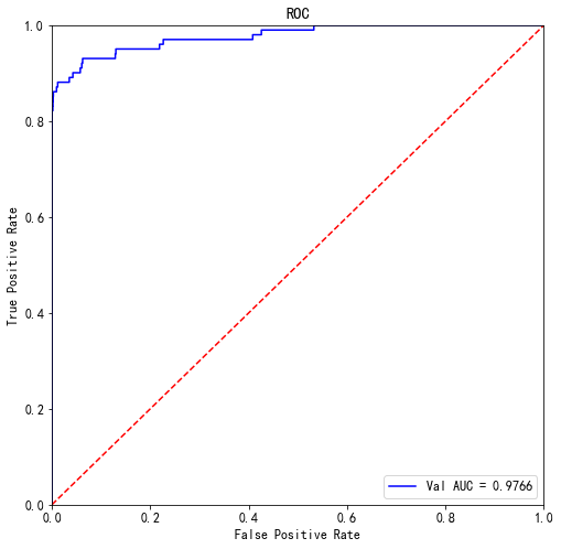
 使用了贝叶斯调参，最后效果索然不如xgboost，但是也比逻辑回归要好，且不需要处理任何变量，直接喂给算法

2021.03.15补充xgboost另外一种调参方式

# -*- coding: utf-8 -*-
"""
Created on Tue Mar  9 16:16:56 2021

@author: Administrator
"""

#%%导入模块
import pandas as pd 
import numpy as np
from scipy import stats
import seaborn as sns
import matplotlib.pyplot as plt
%matplotlib inline
plt.rc("font",family="SimHei",size="12")  #解决中文无法显示的问题


#%%导入数据
creditcard = pd.read_csv('D:/信用卡欺诈检测/creditcard.csv/creditcard.csv')
creditcard.info()


train_y = creditcard[['Class']]
train_y.columns = ['y']
train_x = creditcard.drop(['Class','Time'],axis=1)


import numpy as np
import pandas as pd
import matplotlib.pyplot as plt
import operator
import time
import xgboost as xgb
from xgboost import plot_importance  #画特征重要性的函数
#from imblearn.ensemble import EasyEnsemble  #还有模块木有安装
from sklearn.model_selection import train_test_split
#from sklearn.externals import joblib 已经改成了下面这种方式
import joblib
from sklearn.metrics import auc,roc_curve  #说明是分类
plt.rc('font',family='SimHei',size=13)   #使画出的图形中能正常显示中文
%matplotlib inline


def create_feature_map(features):
    outfile = open('xgb.txt', 'w')  #写，新建一个叫xgb.txt的文件
    i = 0
    for feat in features:
        outfile.write('{0}	{1}	q
'.format(i, feat))   #格式为 0  feature  q  	是分隔符，为空  就是说第一列是序号，第二列是特征名称，第三列是q,不知道需要这个q干吗，可以是多写了，先要着吧，后面再看看吧
        i = i + 1
    outfile.close()
create_feature_map(train_x.columns)

file_xgboost_model='./xgboost_model' #模型文件
file_xgboost_columns='./columns.csv' #最终使用的特征
file_xgboost_model_auc_ks='./xgboost_model_auc_ks.png' #模型AUC和KS值
file_xgboost_model_score='./xgboost_model_score.png' # 模型预测用户的评分分布
file_xgboost_model_prob='./xgboost_model_prob.png' #模型预测用户的概率分布

import xgboost as xgb
from xgboost import XGBClassifier 
from xgboost import plot_tree
import matplotlib.pyplot as plt
from sklearn import metrics
from sklearn.model_selection import train_test_split
from sklearn.metrics import confusion_matrix

X = creditcard.iloc[:,0:-1]
y = creditcard.Class

X_train,X_test,y_train,y_test=train_test_split(X,y,test_size=0.3,random_state=0)

#%%
def tun_parameters(train_x,train_y):  #通过这个函数，确定树的个数
    xgb1 = XGBClassifier(learning_rate=0.1,n_estimators=1000,max_depth=5,min_child_weight=1,gamma=0,subsample=0.8,  
                         colsample_bytree=0.8,objective= 'binary:logistic',scale_pos_weight=1,seed=27)  
    modelfit(xgb1,train_x,train_y)  
 
def modelfit(alg,X, y,useTrainCV=True, cv_folds=5, early_stopping_rounds=50):
    if useTrainCV:
        xgb_param = alg.get_xgb_params()
        xgtrain = xgb.DMatrix(X, label=y)
        cvresult = xgb.cv(xgb_param, xgtrain, num_boost_round=alg.get_params()['n_estimators'], nfold=cv_folds,
            metrics='auc', early_stopping_rounds=early_stopping_rounds,callbacks=[
            xgb.callback.print_evaluation(show_stdv=False),
            xgb.callback.early_stop(early_stopping_rounds)
       ])
        alg.set_params(n_estimators=cvresult.shape[0])
 
    #Fit the algorithm on the data
    alg.fit(X, y,eval_metric='auc')
 
    #Predict training set:
    dtrain_predictions = alg.predict(X)
    dtrain_predprob = alg.predict_proba(X)[:,1]
 
    #Print model report:
    print ("
Model Report")
    print ("Accuracy : %.4g" % metrics.accuracy_score(y, dtrain_predictions))
    print ("AUC Score (Train): %f" % metrics.roc_auc_score(y, dtrain_predprob))
 
    print ('n_estimators=',cvresult.shape[0])
tun_parameters(X_train,y_train)
'''
Accuracy : 0.9998
AUC Score (Train): 0.999886
n_estimators= 100
'''

#%%第二步： max_depth 和 min_child_weight 参数调优
from sklearn.model_selection import GridSearchCV
param_test1 = {
  'max_depth':range(3,10,1),
 'min_child_weight':range(2,9,1)
}
gsearch1 = GridSearchCV(estimator = XGBClassifier(learning_rate =0.1, n_estimators=100, max_depth=5,
min_child_weight=1, gamma=0, subsample=0.8,colsample_bytree=0.8,
 objective= 'binary:logistic', nthread=8,scale_pos_weight=1, seed=27), 
 param_grid = param_test1,scoring='roc_auc',n_jobs=-1,iid=False, cv=5)
gsearch1.fit(X_train,y_train)
gsearch1.best_params_,     gsearch1.best_score_
#({'max_depth': 3, 'min_child_weight': 5}, 0.9851612149724902)
#({'max_depth': 5, 'min_child_weight': 8}, 0.9860796809303931)

#%%第三步：gamma参数调优 
param_test3 = {  
    'gamma': [i / 10.0 for i in range(0, 5)]  
}  
gsearch3 = GridSearchCV(  
    estimator=XGBClassifier(learning_rate=0.1, n_estimators=100, max_depth=5, min_child_weight=8, gamma=0,  
                            subsample=0.8, colsample_bytree=0.8, objective='binary:logistic', nthread=8,  
                            scale_pos_weight=1, seed=27), param_grid=param_test3, scoring='roc_auc', n_jobs=-1,  
    iid=False, cv=5)  
gsearch3.fit(X_train,y_train)  
gsearch3.best_params_, gsearch3.best_score_  
#({'gamma': 0.0}, 0.9860796809303931)
#%%第四步：调整subsample 和 colsample_bytree 参数 
param_test4 = {  
    'subsample': [i / 10.0 for i in range(6, 10)],  
    'colsample_bytree': [i / 10.0 for i in range(6, 10)]  
}  
  
gsearch4 = GridSearchCV(  
    estimator=XGBClassifier(learning_rate=0.1,n_estimators=100, max_depth=5, min_child_weight=8, gamma=0,  
                            subsample=0.8, colsample_bytree=0.8, objective='binary:logistic', nthread=8,  
                            scale_pos_weight=1, seed=27), param_grid=param_test4, scoring='roc_auc', n_jobs=-1,  
    iid=False, cv=5)  
  
gsearch4.fit(X_train,y_train)  
gsearch4.best_params_, gsearch4.best_score_  

#%%第五步：正则化参数调优 reg_alpha和reg_lambda(这里只调了reg_alpha)


def tun_parameters2(train_x,train_y):  #通过这个函数，确定树的个数
    xgb1 = XGBClassifier(learning_rate =0.1, n_estimators=5000, max_depth=5, min_child_weight=8, gamma=0, subsample=0.8, colsample_bytree=0.8,objective= 'binary:logistic', nthread=8,booster='gbtree',
    reg_alpha= 0.6,reg_lambda= 0.8,
    scale_pos_weight=1,seed=2021)
    modelfit(xgb1,train_x,train_y)  
tun_parameters2(X_train,y_train)


'''
Model Report
Accuracy : 0.9997
AUC Score (Train): 0.998747
n_estimators= 134
'''



model = XGBClassifier(base_score=0.5, booster='gbtree', colsample_bylevel=1,
              colsample_bynode=1, colsample_bytree=0.8, gamma=0, gpu_id=-1,
              importance_type='gain', interaction_constraints='',
              learning_rate=0.1, max_delta_step=0, max_depth=5,
              min_child_weight=8, missing=np.nan, monotone_constraints='()',
              n_estimators=134, n_jobs=8, nthread=8, num_parallel_tree=1,
              random_state=27, reg_alpha=0.6, reg_lambda=0.8,
              scale_pos_weight=1, seed=27, subsample=0.8, tree_method='exact',
              validate_parameters=1, verbosity=None)
model.fit(X_train,y_train)  


#%%验证集


def plot_roc(test_x, test_y):
    predictions = model.predict(test_x)
    false_positive_rate, true_positive_rate, thresholds = metrics.roc_curve(test_y, predictions)  #roc的几个参数
    roc_auc = metrics.auc(false_positive_rate, true_positive_rate)  #直接计算auc
    plt.title('Receiver Operating Characteristic')
    plt.plot(false_positive_rate,true_positive_rate, 'b', label='AUC = %0.4f' % roc_auc)
    plt.legend(loc='lower right')
    plt.plot([0, 1], [0, 1], 'r.')
    plt.xlim([0.0, 1.0])
    plt.ylim([0.0, 1.0])
    plt.ylabel('tpr')
    plt.xlabel('fpr')

plot_roc(X_test,y_test)


def run_xgboost(data_x,data_y,random_state_num):
    train_x,valid_x,train_y,valid_y = train_test_split(data_x.values,data_y.values,test_size=0.25,random_state=random_state_num)
    print('开始训练模型')
    start = time.time()
    #转换成xgb运算格式
    d_train = xgb.DMatrix(train_x,train_y)
    d_valid = xgb.DMatrix(valid_x,valid_y)
    watchlist = [(d_train,'train'),(d_valid,'valid')]
    #参数设置（未调箱前的参数）
    params={
        'eta':0.1,                        #特征权重，取值范围0~1，通常最后设置eta为0.01~0.2
        'max_depth':5,                    #树的深度，通常取值3-10，过大容易过拟合，过小欠拟合
        'min_child_weight':8,             #最小样本的权重，调大参数可以繁殖过拟合
        'gamma':0.0,                      #控制是否后剪枝，越大越保守，一般0.1、 0.2的样子
        'subsample':0.8,                  #随机取样比例
        'colsample_bytree':0.8 ,          #默认为1，取值0~1，对特征随机采集比例
        'lambda':0.8,
        'alpha':0.6,
        'n_estimators':500,
        'booster':'gbtree',               #迭代树
        'objective':'binary:logistic',    #逻辑回归，输出为概率
        'nthread':6,                      #设置最大的进程量，若不设置则会使用全部资源
        'scale_pos_weight':10,             #默认为0,1可以处理类别不平衡
        'lambda':1,                       #默认为1，用于L2平滑处理项，避免模型过拟合
        'seed':1234,                      #随机树种子
        'silent':1,                       #0表示输出结果
        'eval_metric':'auc'               #评分指标
    }
    bst = xgb.train(params, d_train,1000,watchlist,early_stopping_rounds=100, verbose_eval=5)   #最大迭代次数1000次
    print(time.time()-start)
    tree_nums = bst.best_ntree_limit
    print('最优模型树的数量：%s,最优迭代次数：%s,auc: %s' %(bst.best_ntree_limit,bst.best_iteration,bst.best_score))
    bst = xgb.train(params, d_train,tree_nums,watchlist,early_stopping_rounds=100, verbose_eval=10) #最优模型迭代次数去训练
    
#     feat_imp = pd.Series(clf.booster().get_fscore()).sort_values(ascending=False)
#     #新版需要转换成dict or list 
#     #feat_imp = pd.Series(dict(clf.get_booster().get_fscore())).sort_values(ascending=False)
#     #plt.bar(feat_imp.index, feat_imp)
#     feat_imp.plot(kind='bar', title='Feature Importances')
    #展示特征重要性排名
    feat_imp = bst.get_fscore(fmap='xgb.txt')
    feat_imp = sorted(feat_imp.items(),key=operator.itemgetter(1))
    df = pd.DataFrame(feat_imp,columns=['feature','fscore'])
    #每个特征被调用的次数/所有特征被调用总次数
    df['fscore'] = df['fscore']/df['fscore'].sum()
    #分数高的排在前面,展示前40个重要特征排名
    df = df.sort_values(by='fscore',ascending=False)
    df = df.iloc[:40]
    plt.figure()
    df.plot(kind='bar',x='feature',y='fscore',legend=True,figsize=(32,10))
    plt.title('XGBoost Feature Importance')
    plt.xlabel('relative importance')
    plt.gcf().savefig('feature_importance_xgb.png')
    plt.show()
    return bst

#%%
# 绘制ROC曲线函数
def plot_roc(test_x, test_y):
    predictions = bst.predict(xgb.DMatrix(test_x))
    false_positive_rate, true_positive_rate, thresholds = roc_curve(test_y, predictions)  #roc的几个参数
    roc_auc = auc(false_positive_rate, true_positive_rate)  #直接计算auc
    plt.title('Receiver Operating Characteristic')
    plt.plot(false_positive_rate,true_positive_rate, 'b', label='AUC = %0.4f' % roc_auc)
    plt.legend(loc='lower right')
    plt.plot([0, 1], [0, 1], 'r.')
    plt.xlim([0.0, 1.0])
    plt.ylim([0.0, 1.0])
    plt.ylabel('tpr')
    plt.xlabel('fpr')

# 绘制K-S函数 从大到小排序，分10等分
def plot_ks(test_x, test_y):
    predictions = bst.predict(xgb.DMatrix(test_x))
    false_positive_rate, true_positive_rate, thresholds = roc_curve(test_y, predictions, drop_intermediate=False)
    pre = sorted(predictions, reverse=True)  #reverse参数为True意味着按照降序排序，这是画ks时要求的
    num = []
    for i in range(10):
        num.append((i) * int(len(pre) / 10))
    num.append(len(pre) - 1)
    df = pd.DataFrame()
    df['false_positive_rate'] = false_positive_rate
    df['true_positive_rate'] = true_positive_rate
    df['thresholds'] = thresholds
    data_ks = []
    for i in num:
        data_ks.append(list(df[df['thresholds'] == pre[i]].values[0]))
    data_ks = pd.DataFrame(data_ks)
    data_ks.columns = ['fpr', 'tpr', 'thresholds']
    ks = max(data_ks['tpr'] - data_ks['fpr'])
    plt.title('K-S曲线')
    plt.plot(np.array(range(len(num))), data_ks['tpr'])
    plt.plot(np.array(range(len(num))), data_ks['fpr'])
    plt.plot(np.array(range(len(num))), data_ks['tpr'] - data_ks['fpr'], label='K-S = %0.4f' % ks)
    plt.legend(loc='lower right')
    plt.xlim([0, 10])
    plt.ylim([0.0, 1.0])
    plt.ylabel('累计占比')
    plt.xlabel('分组编号')

# 绘制一张图，包含训练和测试集的ROC、AUC、K-S图形指标。
def auc_ks(train_x, test_x, train_y, test_y):
    plt.figure(figsize=(15, 15))
    plt.subplot(221)
    plot_roc(train_x, train_y)
    plt.subplot(222)
    plot_roc(test_x, test_y)
    plt.subplot(223)
    plot_ks(train_x, train_y)
    plt.subplot(224)
    plot_ks(test_x, test_y)
    plt.savefig(file_xgboost_model_auc_ks)
    plt.show()

#%%
#保存模型、评价指标、选择变量到D盘
def run_main(data_x,data_y):
    global bst
    start=time.time()
    bst=run_xgboost(data_x,data_y,random_state_num=1234)  #为什么要是1234，因为调参时候就是=1234
    joblib.dump(bst, file_xgboost_model)  #joblib的用法https://www.cnblogs.com/wzdLY/p/9630671.html 将模型保存
    print('模型已成功保存在 %s'%(file_xgboost_model))
    train_x, test_x, train_y, test_y = train_test_split(data_x.values, data_y.values, test_size=0.25, random_state=1234)
    auc_ks(train_x, test_x, train_y, test_y)
    print('模型评价指标已保存在：%s'%(file_xgboost_model_auc_ks))
    print('运行共花费时间：%s'%(time.time()-start))
    resu = bst.predict(xgb.DMatrix(test_x))
    

    

if __name__=='__main__':
    run_main(train_x, train_y)