Partial Order Pruning
2019-CVPR-Partial Order Pruning for Best Speed Accuracy Trade-off in Neural Architecture Search
来源:ChenBong 博客园
- Xin Li (UISEE Tech), Jiashi Feng (NUS, H-index 54)
- GitHub:100+ stars
- https://github.com/lixincn2015/Partial-Order-Pruning
- https://github.com/zym1119/Partial-Order-Pruning-Demo
- Citation:18
Introduction
we propose an algorithm that can offer better speed/accuracy trade-off of searched networks, which is termed “Partial Order Pruning”
提出了speed/accuracy 平衡的网络结构搜索算法“偏序剪枝”算法。
(在特定的平台上,给定延时限制,准确率最高多少?;给定准确率限制,延时最低多少?)
即在给定硬件平台上,找到 Latency/Accuracy trade-off 的边界boundary
It prunes the architecture search space with a partial order assumption
基于“偏序假设”
With the proposed algorithm, we present several Dongfeng (DF) networks that provide high accuracy and fast inference speed on various application GPU platforms.
基于该算法搜索到的“东风网络”,可以在各种GPU平台上分别搜索高精度和快速的网络。
By further searching decoder architectures, our DF-Seg real-time segmentation networks yield state-of-the-art speed/accuracy trade-off on both the target embedded device and the high-end GPU.
通过搜索decoder结构,得到东风分割网络(DF-Seg),可以在嵌入式设备和GPU上都取得SOTA的speed/accuracy 平衡的模型
Motivation
Deploying deep convolutional neural networks (CNNs) on real-world embedded devices
在实际的嵌入式设备上部署CNNs
Despite the considerable efforts on accelerating inference of CNNs such as pruning [11], quantization [29] and factorization [17], fast inference speed is usually achieved at the cost of degraded performance [22, 15].
尽管有了很多的加速方法(剪枝,量化,分解),但通常是以精度下降为代价
In this paper, we address such a practical problem: Given a target platform, what is the best speed/accuracy trade-off boundary curve by varying CNN architecture?
本文要解决2个实际问题:在给定的平台上,找到speed/accuracy 平衡的边界
Or more specifically, we aim to answer two questions: 1) Given the maximum acceptable latency, what is the best accuracy one can get? 2) To meet certain accuracy requirements, what is the lowest inference latency one can expect?
具体地,给定延时限制,最高的准确率多少?给定准确率限制,最低的延时多少?
Some existing works manually design high accuracy network architectures [33, 31, 13, 25].They usually adopt an indirect metric, i.e. FLOP, to estimate the network complexity, but the FLOP count does not truly reveal the actual inference speed.
一些工作只考虑FLOPs的指标,但FLOP不代表实际的推理速度。
For example, for a 3 × 3 convolution on Nvidia GPUs which is highly optimized in terms of both hardware and software design [16], one can assume it is 9 times slower than a 1 × 1 convolution on GPUs since it has 9 times more FLOPs, which is not true actually.
例如 使用FLOP计算的话,3 × 3 卷积比1 × 1卷积慢9倍;实际上 3 × 3 卷积在Nvidia GPUs 上有着高度的软硬件优化,因此3 × 3 卷积实际速度很快。
Besides, another important factor that affects the inference speed, the memory access, is not covered by measuring FLOPs.
另一个影响实际速度的重要因素是,memory access(显存访问?)不能被FLOPs衡量。
Considering the diversities of hardware and software, it is almost impossible to find one single architecture that is optimal for all the platforms.
考虑到设备的多样性,几乎不可能找到适合所有设备的单一网络架构。
Some other works attempt to automatically search for the optimal network architecture [36, 23, 19], but they also rely on FLOPs to estimate the network complexity and do not take into account the discrepancy of this metric with the actual inference speed and also the target platforms.
一些NAS工作自动搜索最佳结构,但也是使用FLOPs估计网络复杂度。
Despite a few works [8, 2, 28] consider the actual inference speed on target platforms, they search the architecture in each individual building block and keep fixed the overall architecture, i.e. depth and width.
其他一些NAS工作考虑到特定平台的推理速度,但他们是固定模型的深度和宽度,而搜索每个block的结构。
In this paper, we develop an efficient architecture search algorithm that automatically selects the networks that offer better speed/accuracy trade-off on a target platform.
The proposed algorithm is termed “Partial Order Pruning”, with which some candidates that fail to give better speed/accuracy trade-off are filtered out at early stages of the architecture searching process based on a partial order assumption (see Section 3.3 for details).
For example, a wider network cannot be more efficient than a narrower one with the same depth, thus accordingly some wider ones are discarded.
By pruning the search space in this way, our algorithm is forced to concentrate on those architectures that are more likely to lift the boundary of speed/accuracy tradeoff.
Contribution
We are among the first to investigate the problem of balancing speed and accuracy of network architectures for network architecture search.
我们第一个开始研究特定平台上的speed/accuracy trade-off 的网络结构搜索问题。
By pruning the search space with a partial order assumption, our “Partial Order Pruning” algorithm can efficiently lift the boundary of speed/accuracy trade-off.
通过“偏序剪枝算法”可以有效地找到speed/accuracy边界
We present several DF networks that provide both high accuracy and fast inference speed on target embedded device TX2.
东风网络可以在嵌入式设备TX2上,同时达到高准确率与快的推理速度。
The accuracy of our DF1/DF2A networks exceeds ResNet18/50 on ImageNet validation set, but the inference latency is 43% and 39% lower, respectively.
DF1/DF2A在ImageNet上的准确率分别超过ResNet18/50,延时分别低了43%和39%。
We apply the proposed algorithm to searching decoder architectures for a segmentation network.
Together with DF backbone networks, we achieve new stateof-the-art in real-time segmentation on both high-end GPUs and target embedded device TX2.
On GTX 1080Ti, our DF1-Seg network achieves 106.4 FPS at resolution 1024×2048 with mIoUclass 74.1%. On TX2, our DF1-Seg network achieves 21.8 FPS at resolution 1280 × 720, i.e. 720p.
Method
Search Space 搜索空间
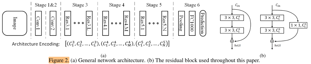
We provide a general network architecture in our search space, as shown in Figure 2(a).
Stages 1∼5 down-sample the spatial resolution of the input tensor with a stride of 2, and stage 6 produces the final prediction with a global average pooling and a fully connected layer.
搜索空间分为6个阶段(如图2),stages 1~5是stride=2的下采样阶段,Stage1/2各是一个卷积层,Stage 6是Pooling层、FC1000层。stage1, 2, 6结构是固定的,stage 3, 4, 5 是需要搜索的部分。
For stages 3, 4, 5, each consists of L, M, N residual blocks, Different settings of L/M/N lead to different network depths.
Stage 3, 4, 5分别有L, M, N 个Residual Blocks 组成,L, M, N表示深度。
The width (number of channels) of the i-th residual block in stage s is denoted as (C_s^i) ,In practice, we restrict (C_s^i) ∈ {64, 128, 256, 512, 1024}
每个Residual Block 都有不同的宽度,第s个stage的第i个 Residual Block的宽度表示为 (C_s^i) ,取值限制在 (C_s^i) ∈ {64, 128, 256, 512, 1024}
对于搜索空间之中的每个网络,我们都使用了一个字符串去编码它的结构,如 [(64,64), (128, 256), (256)] 就表示了stage 3有两层,宽度64,stage 4有2层,宽度128和256,stage 5有一层,宽度256 。
We empirically restrict the width of a block to be no narrower than its preceding blocks.
我们人为规定了规则,后一个块的宽度不能低于前一个块,即保证网络的通道数是一个单调不减序列。
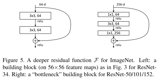
As shown in Figure 2(b), the building block consists of two convolution layers and a shortcut connection. An additional projection layer is added if the size of input does not match the output tensor.
一个Residual Block由2个卷积层和1个shortcut 组成(图2b左),如果输入通道和输出的通道数不匹配,则附加一个1×1的 projection layer(图2b右)
All convolutional layers are followed with a batch normalization [14] layer and ReLU nonlinearity.
所有的卷积层后都跟着BN层和ReLU层。
Latency Estimate 延时估计
The set of all possible architectures, with different depths (number of blocks) and widths (number of channels per block), is denoted as S and usually referred to as the search space in neural architecture search [19, 36].
不同的深度和宽度的网络构成整个搜索空间 (S) ,搜索空间无限大。
The latency of architectures in S can vary from very small to positive infinity.
But we only care about architectures in a subspace (hat S subset S) , which provide latency in the range [Tmin, Tmax].
但我们只需要考虑推理时间在[$T_{min}, T_{max} $]区间内的子空间 (hat S) 即可,这是因为我们关注的性能指标就是特定平台上的推理时间,我们并不需要在该平台下推理时间过长的模型。
Thus we can construct a look-up table Latency (ci, hi, wi, co, ho, wo) providing latency of each block configuration, where ci/co is the number of channels in input/output tensor, and hi/wi/ho/wo is the corresponding spatial size.
For example, Latency (32, 112, 112, 64, 56, 56) = 0.143ms on TX2.
By simply summing up the latency of all blocks, we can efficiently estimate the latency Lat(x) of an architecture x ∈ S.
对于推理时间,我们与FBNet、ProxylessNAS的方法不谋而合,均是通过查找表去预测。构建查找表,输入一个Residual Block的参数 (ci, hi, wi, co, ho, wo) 就能得到这个Block的延时,将所有block的延时累加后就是整个网络的总延时。
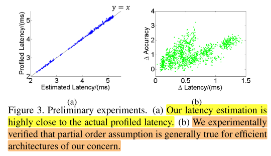
In Figure 3(a), we compare the estimated latency with the profiled latency. It shows our latency estimation is highly close to the actual profiled latency.
实验发现这种方法确实是非常的稳定(图3a)。
Partial Order Assumption 偏序假设
A partial order is a binary relation defined over a set. It means that for certain pairs of elements (x, y) in the set, one of the elements x precedes the other y in the ordering, denoted with x ≺ y.
Here “partial” indicates that not every pair of elements needs to be comparable.
偏序关系是集合元素之间的二元关系,元素x排在y之前,记为x < y, 读作x小于y。“偏序”意味着不是每2个元素之间都可以比较,只有部分元素之间可以比较。
We find that there is a partial order relation among architectures in our search space.
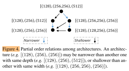
In Figure 4, we follow the architecture encoding in Figure 2(a), and illustrate the partial order relation among architectures.
我们发现搜索空间内的结构编码之间存在偏序关系,如图2a
Let x, y ∈ (hat S) denote two elements in the set (hat S) . If x is shallower than y but they are with the same width, or narrower than y with same depth, we can borrow the concept from the order theory, and say that x precedes y in the ordering, denoted as x ≺ y. In the rest of this paper, we also call x a precedent of y if x ≺ y.
x, y是搜索子空间 (hat S) 中的元素,若x的深度 < y的深度,但宽度相同;或者x的宽度 < y的宽度,但深度相同;我们说x排在y之前,记为x<y.
Let Acc(x) and Lat(x) denote the accuracy and latency of the architecture x.
Then the partial order assumption of architectures can be summarized as
Lat(x) ≤ Lat(y), Acc(x) ≤ Acc(y), (1)
where ∀x, y ∈ (hat S) , x ≺ y.
Acc(x) and Lat(x) 分别表示结构x的准确率和延时,我们提出结构的偏序假设,若x<y,则x的延时低于y,x的准确率低于y。
This assumption may not hold for very deep networks that contain hundreds of layers [12], but it is generally true for the efficient architectures of our concern, i.e. (hat S) , which is experimentally verified in this work.
这个假设对于非常深的几百层网络不一定成立,但当网络层数较小时基本成立,如我们的搜索空间 (hat S)。
We find all comparable architecture pairs (x, y), x ≺ y in our trained architectures (Section 4.2), and compute the latency difference ∆Lat = Lat(y) − Lat(x) and accuracy difference ∆Acc = Acc(y) − Acc(x) in each pair.
我们找了一些偏序对(x, y), x < y, 做了实验,计算 ∆Lat = Lat(y) − Lat(x) ∆Acc = Acc(y) − Acc(x),(若假设成立,则Lat(y) > Lat(x),且 Acc(y) > Acc(x),即 ∆Lat > 0 且 ∆Acc >0。
As shown in Figure 3(b), most points locate in the first quartile. This means the accuracy of the precedent x is lower, for almost all comparable pairs.
如图3b,绝大部分点都在第一象限(即 ∆Lat > 0 且 ∆Acc >0),说明假设有效。
This assumption can be utilized to prune the architecture search space, and speed up the search process significantly.
偏序假设可以用来修剪搜索空间,加速搜索进程。
Partial Order Pruning 偏序剪枝
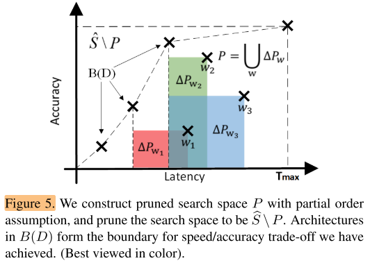
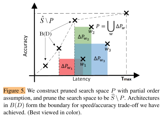
以上图为例,搜索空间中每一个点都对应着上图坐标系中的一个模型。我们对找到的每一个w,都希望能得到与其相关的需要剪枝掉的搜索空间 (P_w) , (P_w) 代表着无论是速度还是精度都不如w的模型们,但是 (P_w) 这部分包含的模型究竟是什么样的呢?我们不知道。而且, (P_w) 虽然位于w的左下区域,但并不代表分布于w左下的所有模型我们都不需要,Pw需要一个下界,否则我们可能剪掉了低延时下的边界模型。虽然 (P_w) 我们不知道,但是 (P_w) 中的一部分模型我们是知道的,这一部分就是和w存在偏序关系的模型,因为这些模型在图中的分布情况可以通过w进行估计。
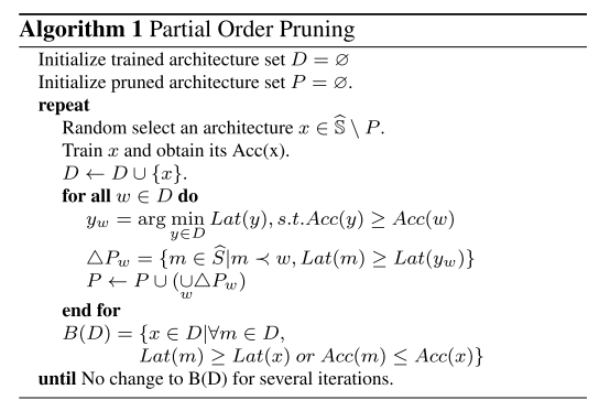
最终整体的算法流程可以总结为:
初始化已训练模型集合D=∅,剪掉的模型集合P=∅
1、从搜索空间( (hat S) P,搜索空间为[(T_{min}, T_{max})] 的子空间 (hat S) 去掉P中的元素)中随机采样w
2、训练w,得到性能和估计的推理时间,将w加入已训练集合D
3、遍历已训练集合D,找到准确率最高,同时速度最快的模型 (y_w) , (y_w) 的延时将会是 (P_w) 的下界
4、根据 w和 延时下界 得到剪掉的模型集合 (P_w) ,即与w存在偏序关系,可以估计出既不如w也不如 (y_w) 的模型集合
5、从搜索空间中删除 (P_w) 模型(将 (P_w) 并入P,并回到步骤1,直到边界模型在一定迭代次数后不再更新
Partial Order Pruning不仅可以搜索classification的模型,加上decoder也可以搜索出一个segmentation的模型。
Experiments
We adopt two typical kinds of hardware that provide different computational power.
Embedded device: We use Nvidia Jetson TX2
High-end GPU: We use Nvidia Geforce GTX 1080Ti
实验使用了2种设备,嵌入式设备TX2,GPU 1080Ti
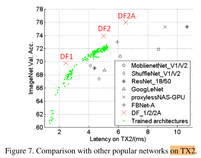
We train ∼ 200 networks in total, as shown in Figure 7.
The resulting models are referred to as DF1, DF2.
我们训练了大约200个网络,得到2个网络结构DF1,DF2。
We further replace some of the building blocks in DF2 from basic block in Figure 2(b) to bottleneck block [12],The resulting network is denoted as DF2A.
进一步将DF2的block替换为bottleneck block,得到DF2A
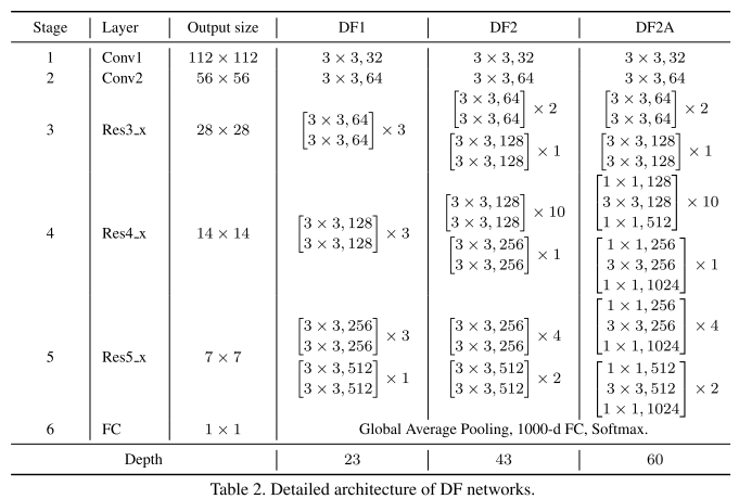
Table 2 shows detailed architectures of these three DF networks.
表2展示了三种DF网络的结构细节
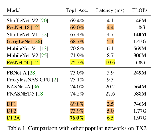
与经典网络对比:
Compared with ResNet-18 and GoogLeNet, our DF1 obtains a higher accuracy 69.8% but the inference latency is 43%, 51% lower than two baselines respectively.
our DF2 has a similar latency but the accuracy is 4.9% and 5.2% higher than the baselines respectively.
Furthermore, DF2A achieves a surpassing ResNet-50-level accuracy with a 39% lower latency.
Note we use the same building blocks with ResNet-18/50. So we attribute the better speed/accuracy trade-off to the better balancing between depth and width in our architectures.
注意我们使用的是与ResNet-18/50相同的block,因此达到更好地speed/accuracy 平衡的原因是更好地平衡了深度和宽度。
与小网络对比:
MobileNet [13, 25] and ShuffleNet [32, 20] are stateof-the-art efficient networks that are designed for mobile applications.
We also compare our DF networks to them on TX2 in Table 1 and Figure 7.
It can be seen our DF1 achieves higher accuracy but lower inference latency.
This is because they have higher memory access cost. The total memory cost (i.e. intermediate features) for ShuffleNet V2 and DF1 is 4.86M and 2.91M respectively.
This also indicates the FLOPs may be inconsistent with latency on the target platform [27, 20].
与NAS方法对比:
We also compare our DF networks with other models searched by NAS methods [36, 18, 28, 2].
As shown in Table 1, NASNet [36] and PNASNet [18] have not taken latency into consideration, leading to higher latency.
Comparing to FBNet [28] and ProxylessNAS [2], which also take target platform-related objectives into neural architecture search, our DF networks show better speed/accuracy tradeoff.
This can be explained as (a) DF networks are specifically searched for TX2 platform; (b) FBNet and ProxylessNAS use an inverted bottleneck module, which brings more memory access cost; (c) FBNet and ProxylessNAS aim at searching for better building block architectures while we balance the width and depth of the overall architecture.
发现:
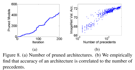
We then discuss the search efficiency of our proposed algorithm. Figure 8(a) shows the number of pruned architectures in the search process.
We prune 438 architectures after training 200 architectures.Therefore, our POP algorithm accelerates the architecture search process for 2.2 times.
搜索效率,如图8a,横坐标为训练的模型结构数,纵轴为剪掉的模型结构数,在训练200个结构时,剪掉了438个结构,说明“偏序剪枝”算法大约有2.2倍的搜索加速比。
Each model takes 5 ∼ 7 hours on a server with 8-GPUs. Training 200 architectures takes ∼ 400 GPU days in total.
The computational cost of our architecture for searching on ImageNet is lower than the building block architecture searching [36, 23] on CIFAR-10 by an order.
每个结构需要在8卡的GPU机器上训练5-8个小时,一共训练200个结构,总共需要大致400个GPU days,我们是在ImageNet上进行搜索,比一些在CIFAR-10上搜索的NAS方法所需的时间还要少。
Based on our architecture search results, we make following observations.
Very quick down-sampling is preferred in early stages to obtain higher efficiency. We use 1 convolutional layer in each of stages 1&2, and are still able to achieve good accuracy.
Down-sampling with the convolutional layer is preferred to the pooling layer for obtaining higher accuracy. We only use 1 global average pooling at the end of the network.
We empirically find that the accuracy of a network is correlated to the number of its precedents, as shown in Figure 8(b).
We assume that an architecture with more precedents may have a better balance between depth and width.
- 在早期最好使用下采样,可以提高效率。前2个阶段只使用2个卷积层,仍然可以达到很好的精度
- 卷积层的下采样和池化的下采样相比,卷积层的下采样更好,我们只在网络末端使用1个全局平均池化层。
- 实验发现,网络的准确率与网络的先序结构数量相关(图8b)。
Conclusion
We propose a network architecture search algorithm “Partial Order Pruning” , which is able to lift the boundary of speed/accuracy trade-off of searched networks on the target platform.
By utilizing a partial order assumption, it efficiently prunes the feasible architecture space to speed up the search process.
The searched DF backbone newtorks provide state-of-the-art speed/accuracy trade-off on target platforms.
Summary
感觉这篇文章有意思,这个文章不是在FLOPs这些传统的指标下硬磕,而是找了一个新的评价体系——在特定机器上比延时,相同延时下精度更高(因为模型的FLOPs大,精度高很正常)感觉像是降维打击。就是绕开传统的比较指标,自创一个新的评价体系来对比。
Reference
【CVPR2019 | Partial Order Pruning - 特定平台下的高效网络结构搜索】https://zhuanlan.zhihu.com/p/69852042
【Paper Reading - Partial Order Pruning】https://zhuanlan.zhihu.com/p/68395137