Tensorflow实现各种学习率衰减
觉得有用的话,欢迎一起讨论相互学习~


学习率衰减(learning rate decay)
- 加快学习算法的一个办法就是随时间慢慢减少学习率,我们将之称为学习率衰减(learning rate decay)
概括
- 假设你要使用mini-batch梯度下降法,mini-batch数量不大,大概64或者128个样本,但是在迭代过程中会有噪音,下降朝向这里的最小值,但是不会精确的收敛,所以你的算法最后在附近摆动.,并不会真正的收敛.因为你使用的是固定的 (alpha),在不同的mini-batch中有杂音,致使其不能精确的收敛.

- 但如果能慢慢减少学习率 (alpha) 的话,在初期的时候,你的学习率还比较大,能够学习的很快,但是随着 (alpha) 变小,你的步伐也会变慢变小.所以最后的曲线在最小值附近的一小块区域里摆动.所以慢慢减少 (alpha) 的本质在于在学习初期,你能承受较大的步伐, 但当开始收敛的时候,小一些的学习率能让你的步伐小一些.

细节
- 一个epoch表示要遍历一次数据,即就算有多个mini-batch,但是一定要遍历所有数据一次,才叫做一个epoch.
- 学习率 (alpha ,其中 alpha_{0}表示初始学习率, decay-rate是一个新引入的超参数) :

其他学习率是衰减公式
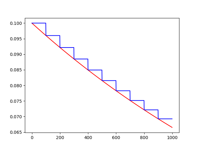
指数衰减
Tensorflow实现学习率衰减
自适应学习率衰减
tf.train.exponential_decay(learning_rate, global_step, decay_steps, decay_rate, staircase=False, name=None)
退化学习率,衰减学习率,将指数衰减应用于学习速率。
计算公式:
decayed_learning_rate = learning_rate * decay_rate ^ (global_step / decay_steps)
# 初始的学习速率是0.1,总的迭代次数是1000次,如果staircase=True,那就表明每decay_steps次计算学习速率变化,更新原始学习速率,
# 如果是False,那就是每一步都更新学习速率。红色表示False,蓝色表示True。
import tensorflow as tf
import numpy as np
import matplotlib.pyplot as plt

learning_rate = 0.1  # 初始学习速率时0.1
decay_rate = 0.96  # 衰减率
global_steps = 1000  # 总的迭代次数
decay_steps = 100  # 衰减次数

global_ = tf.Variable(tf.constant(0))
c = tf.train.exponential_decay(learning_rate, global_, decay_steps, decay_rate, staircase=True)
d = tf.train.exponential_decay(learning_rate, global_, decay_steps, decay_rate, staircase=False)

T_C = []
F_D = []

with tf.Session() as sess:
   for i in range(global_steps):
       T_c = sess.run(c, feed_dict={global_: i})
       T_C.append(T_c)
       F_d = sess.run(d, feed_dict={global_: i})
       F_D.append(F_d)

plt.figure(1)
plt.plot(range(global_steps), F_D, 'r-')# "-"表示折线图,r表示红色,b表示蓝色
plt.plot(range(global_steps), T_C, 'b-')
# 关于函数的值的计算0.96^(3/1000)=0.998
plt.show()
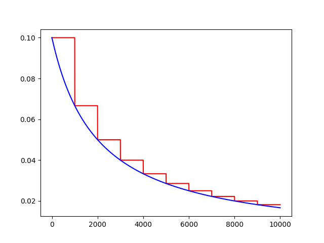
反时限学习率衰减
inverse_time_decay(learning_rate, global_step, decay_steps, decay_rate,staircase=False,name=None)
将反时限衰减应用到初始学习率。
计算公式:
decayed_learning_rate = learning_rate / (1 + decay_rate * t)
import tensorflow as tf
import matplotlib.pyplot as plt

global_ = tf.Variable(tf.constant(0), trainable=False)
globalstep = 10000  # 全局下降步数
learning_rate = 0.1  # 初始学习率
decaystep = 1000  # 实现衰减的频率
decay_rate = 0.5  # 衰减率

t = tf.train.inverse_time_decay(learning_rate, global_, decaystep, decay_rate, staircase=True)
f = tf.train.inverse_time_decay(learning_rate, global_, decaystep, decay_rate, staircase=False)

T = []
F = []

with tf.Session() as sess:
    for i in range(globalstep):
        t_ = sess.run(t, feed_dict={global_: i})
        T.append(t_)
        f_ = sess.run(f, feed_dict={global_: i})
        F.append(f_)

plt.figure(1)
plt.plot(range(globalstep), T, 'r-')
plt.plot(range(globalstep), F, 'b-')
plt.show()
学习率自然指数衰减
def natural_exp_decay(learning_rate, global_step, decay_steps, decay_rate, staircase=False, name=None)
将自然指数衰减应用于初始学习速率。
计算公式:
decayed_learning_rate = learning_rate * exp(-decay_rate * global_step)
import tensorflow as tf
import matplotlib.pyplot as plt

global_ = tf.Variable(tf.constant(0), trainable=False)
globalstep = 10000  # 全局下降步数
learning_rate = 0.1  # 初始学习率
decaystep = 1000  # 实现衰减的频率
decay_rate = 0.5  # 衰减率

t = tf.train.natural_exp_decay(learning_rate, global_, decaystep, decay_rate, staircase=True)
f = tf.train.natural_exp_decay(learning_rate, global_, decaystep, decay_rate, staircase=False)

T = []
F = []

with tf.Session() as sess:
    for i in range(globalstep):
        t_ = sess.run(t, feed_dict={global_: i})
        T.append(t_)
        f_ = sess.run(f, feed_dict={global_: i})
        F.append(f_)

plt.figure(1)
plt.plot(range(globalstep), T, 'r-')
plt.plot(range(globalstep), F, 'b-')
plt.show()

常数分片学习率衰减
piecewise_constant(x, boundaries, values, name=None)
例如前1W轮迭代使用1.0作为学习率,1W轮到1.1W轮使用0.5作为学习率,以后使用0.1作为学习率。
import tensorflow as tf
import numpy as np
import matplotlib.pyplot as plt

# 当global_取不同的值时learning_rate的变化,所以我们把global_
global_ = tf.Variable(tf.constant(0), trainable=False)
boundaries = [10000, 12000]
values = [1.0, 0.5, 0.1]
learning_rate = tf.train.piecewise_constant(global_, boundaries, values)
global_steps = 20000

T_L = []
with tf.Session() as sess:
    for i in range(global_steps):
        T_l = sess.run(learning_rate, feed_dict={global_: i})
        T_L.append(T_l)

plt.figure(1)
plt.plot(range(global_steps), T_L, 'r-')
plt.show()

多项式学习率衰减
特点是确定结束的学习率。
polynomial_decay(learning_rate, global_step, decay_steps,end_learning_rate=0.0001, power=1.0,cycle=False, name=None):
通常观察到,通过仔细选择的变化程度的单调递减的学习率会产生更好的表现模型。此函数将多项式衰减应用于学习率的初始值。
使学习率learning_rate在给定的decay_steps中达到end_learning_rate。它需要一个global_step值来计算衰减的学习速率。你可以传递一个TensorFlow变量,在每个训练步骤中增加global_step = min(global_step, decay_steps)
计算公式:
decayed_learning_rate = (learning_rate - end_learning_rate) *(1 - global_step / decay_steps) ^ (power) + end_learning_rate
如果cycle为True,则使用decay_steps的倍数,第一个大于'global_steps`.ceil表示向上取整.
decay_steps = decay_steps * ceil(global_step / decay_steps)
decayed_learning_rate = (learning_rate - end_learning_rate) *(1 - global_step / decay_steps) ^ (power) + end_learning_rate
Example: decay from 0.1 to 0.01 in 10000 steps using sqrt (i.e. power=0.5):'''
import tensorflow as tf
import matplotlib.pyplot as plt

global_ = tf.Variable(tf.constant(0), trainable=False)
starter_learning_rate = 0.1  # 初始学习率
end_learning_rate = 0.01  # 结束学习率
decay_steps = 1000
globalstep = 10000
f = tf.train.polynomial_decay(starter_learning_rate, global_, decay_steps, end_learning_rate, power=0.5, cycle=False)
t = tf.train.polynomial_decay(starter_learning_rate, global_, decay_steps, end_learning_rate, power=0.5, cycle=True)
F = []
T = []
with tf.Session() as sess:
    for i in range(globalstep):
        f_ = sess.run(f, feed_dict={global_: i})
        F.append(f_)
        t_ = sess.run(t, feed_dict={global_: i})
        T.append(t_)

plt.figure(1)
plt.plot(range(globalstep), F, 'r-')
plt.plot(range(globalstep), T, 'b-')
plt.show()
