How the production environment at Google fits together for networking, monitoring and finishing with a sample service architecture at Google.
I am a Site Reliability Engineer at Google, annotating the SRE book in a series of posts. The opinions stated here are my own, not those of my company.
This is the second half of Chapter 2: The Production Environment at Google, from the Viewpoint of an SRE.
Networking
Google’s network hardware is controlled in several ways. As discussed earlier, we use an OpenFlow-based software-defined network. Instead of using “smart” routing hardware, we rely on less expensive “dumb” switching components in combination with a central (duplicated) controller that precomputes best paths across the network. Therefore, we’re able to move compute-expensive routing decisions away from the routers and use simple switching hardware.
Just to clarify here: This is specifically talking about Google’s usage of its own networking gear to create an international high bandwidth network to transmit data between its own datacenters. To connect with network peers, “traditional” equipment is used.
Network bandwidth needs to be allocated wisely. Just as Borg limits the compute resources that a task can use, the Bandwidth Enforcer (BwE) manages the available bandwidth to maximize the average available bandwidth. Optimizing bandwidth isn’t just about cost: centralized traffic engineering has been shown to solve a number of problems that are traditionally extremely difficult to solve through a combination of distributed routing and traffic engineering [Kum15].
I’m going to put this reference on my reading list: A. Kumar et al., “BwE: Flexible, Hierarchical Bandwidth Allocation for WAN Distributed Computing”, in SIGCOMM ‘15.
Some services have jobs running in multiple clusters, which are distributed across the world. In order to minimize latency for globally distributed services, we want to direct users to the closest datacenter with available capacity. Our Global Software Load Balancer (GSLB) performs load balancing on three levels:
GSLB is our layer of abstraction that lets any service at Google talk to any other service at Google, providing addressing, capacity management, overload protection, monitoring, health checking, and is just generally amazing. Lets go through its 10,000 foot view:
Geographic load balancing for DNS requests (for example, to www.google.com),described in Load Balancing at the Frontend
Lots of internet companies do this. This is the simplest way of getting traffic in Australia to be served from Australia, and traffic from London being served in Europe.
It of course goes wrong a little of the time. Getting a tiny amount of traffic from Japan served from somewhere in Africa is rather negative and might happen, but that’s a price you pay. :)
Load balancing at a user service level (for example, YouTube or Google Maps)
Unlike the DNS approach above, this and the next part are for all services inside Google as well as outside. Where DNS is only used for internet traffic heading towards Google.
Load balancing at the Remote Procedure Call (RPC) level, described in Load Balancing in the Datacenter
Do you ever wish that your clients knew which server had the capacity to serve your request, instead of finding out via a 503/504 that it’s overloaded? That’s something that we get with GSLB. The clients themselves are smart enough to know to direct the right amount of traffic to the less-used, further-away, backends.
Service owners specify a symbolic name for a service, a list of BNS addresses of servers, and the capacity available at each of the locations (typically measured in queries per second). GSLB then directs traffic to the BNS addresses.
“Typically” measured in queries per second. That’s because I haven’t caught them and asked the team who owns the service to justify why they’re not measuring utilization and balancing traffic as according to the available capacity.
At Google it used to be that GSLB could only balance based on the queries per second (QPS) of a backend cluster. Since then it has been engineered to require much less maintenance and be more reliable, by measuring in real-time the CPU usage of all the servers in each cluster, and balancing as according to their real capacity updated in real-time.
The Google Cloud Platform product “Google Cloud Load Balancer” is an externalised version of GSLB, which can be easily configured to read the CPU usage of your backends in the way that I describe.
Other System Software
Several other components in a datacenter are also important.
Lock Service
I think this section misses the point about what chubby is useful for or why it’s important.
The Chubby [Bur06] lock service provides a filesystem-like API for maintaining locks. Chubby handles these locks across datacenter locations. It uses the Paxos protocol for asynchronous Consensus (see Managing Critical State: Distributed Consensus for Reliability).
Chubby stores small amounts of data with strong consistency.
Chubby also plays an important role in master election. When a service has five replicas of a job running for reliability purposes but only one replica may perform actual work, Chubby is used to select which replica may proceed.
This fact is presented in the Google SRE new employee training. And it has never once been useful to me. I don’t know why we say it there, I don’t know why it’s mentioned here.
Data that must be consistent is well suited to storage in Chubby. For this reason, BNS uses Chubby to store mapping between BNS paths and IP address:portpairs.
Addressing being strongly consistent is convenient, so we store it in our system that stores small amounts of data with strong consistency. But addresses don’t need to be strongly consistent, it’s just kinda convenient, and at Google we rely on it, instead of using other equally valid techniques that have different trade-offs.
This doesn’t say anything about how we make chubby into an extremely scalable platform for storing and publishing data, which is actually important, because if you tried to use a master election(!) system to store important information like server addresses in a Google-scale datacenter network, it would explode nearly immediately.
Monitoring and Alerting
We want to make sure that all services are running as required. Therefore, we run many instances of our Borgmon monitoring program (see Practical Alerting from Time-Series Data). Borgmon regularly “scrapes” metrics from monitored servers. These metrics can be used instantaneously for alerting and also stored for use in historic overviews (e.g., graphs). We can use monitoring in several ways:
Every single server at Google has a standard way of reporting monitoring metrics. It doesn’t matter which language it’s implemented in, or if it’s a batch job, rpc service or web server. This is a very powerful standard that allows someone an engineer who knows literally nothing about the job, but read the monitoring telemetry and make intelligent decisions.
Set up alerting for acute problems.
Sudden 10% error rate? We have a multitude of standard rules that we can apply to the standard metrics, or we can write our own rules that apply to custom metrics that only specific jobs publish. These typically cause pagers to go off, or bugs to be filed.
Compare behavior: did a software update make the server faster?
Your system has a baseline 0.01% error rate on previous binary, but 0.9% on the servers with the new binary. Rollback the release!
When you tell Borg to update a job to have new settings or a new binary, the standard metrics for error rates and such are inspected part-way through to see jumps in error rates, and automatically trigger a roll back.
Improving the server updater in this way was done by an SRE who decided that the idea of a human looking at a graph to verify that a rollout was working correctly was the wrong way to do things. This is exactly the sort of clear win that SRE team members should be looking out for in their systems.
Examine how resource consumption behavior evolves over time, which is essential for capacity planning.
I referred to this in a previous post. We feed historical monitoring data into some pretty sophisticated algorithms to do capacity planning. But sometimes we also just eyeball a graph
Our Software Infrastructure
Our software architecture is designed to make the most efficient use of our hardware infrastructure. Our code is heavily multithreaded, so one task can easily use many cores. To facilitate dashboards, monitoring, and debugging, every server has an HTTP server that provides diagnostics and statistics for a given task.
I did refer to one aspect of this in the previous section about monitoring.
All of Google’s services communicate using a Remote Procedure Call (RPC) infrastructure named Stubby; an open source version, gRPC, is available. Often, an RPC call is made even when a call to a subroutine in the local program needs to be performed. This makes it easier to refactor the call into a different server if more modularity is needed, or when a server’s codebase grows. GSLB can load balance RPCs in the same way it load balances externally visible services.
Imagine never having to learn a new API for each new service. Checking if it’s XML, XML-RPC, SOAP, REST, or any other random format. That’s what it’s like at Google. Everything talks to everything else over a single RPC framework with a consistent addressing scheme.
A server receives RPC requests from its frontend and sends RPCs to its backend. In traditional terms, the frontend is called the client and the backend is called the server.
Every frontend is a backend to someone. It’s frontends and backends all the way down until you have no backends of your own…. I have to use this terminology, but it does cause a considerable amount of confusion when you talk to someone who thinks about your server from a different perspective.
Data is transferred to and from an RPC using protocol buffers, often abbreviated to “protobufs,” which are similar to Apache’s Thrift. Protocol buffers have many advantages over XML for serializing structured data: they are simpler to use, 3 to 10 times smaller, 20 to 100 times faster, and less ambiguous.
Protocol buffers are used everywhere at Google. They’re the universal data exchange and storage format. Used for data in flight and data at rest. Google even has specialized distributed query mechanisms so you can have billions of protocol buffers and query them using BigQuery, in mere minutes instead of hours.
A typical Google engineer could describe their job as “Taking protocol buffers and turning them into other protocol buffers” and be entirely accurate about what they do all day.
Our Development Environment
Development velocity is very important to Google, so we’ve built a complete development environment to make use of our infrastructure [Mor12b].
Mor12b is: J. D. Morgenthaler, M. Gridnev, R. Sauciuc, and S. Bhansali, “Searching for Build Debt: Experiences Managing Technical Debt at Google”, in Proceedings of the 3rd Int’l Workshop on Managing Technical Debt, 2012.
Apart from a few groups that have their own open source repositories (e.g., Android and Chrome), Google Software Engineers work from a single shared repository [Pot16]. This has a few important practical implications for our workflows:
If engineers encounter a problem in a component outside of their project, they can fix the problem, send the proposed changes (“changelist,” or CL) to the owner for review, and submit the CL to the mainline.
Whenever you read “CL” or “Changelist” you may mentally replace it with “PR” / “Pull Request”. They’re functionally equivalent.
Changes to source code in an engineer’s own project require a review. All software is reviewed before being submitted.
I do a higher-than-average number of code reviews. It all starts to blur together, but I can now spot a bad idiom, a poor library choice, or a trailing newline at 100 yards.
This felt very onorous when I first came to Google from a smaller company, but now it feels very natural, and I always appreciate having an extra pair (or few pairs) of eyes on every line of code I write.
When software is built, the build request is sent to build servers in a datacenter. Even large builds are executed quickly, as many build servers can compile in parallel. This infrastructure is also used for continuous testing. Each time a CL is submitted, tests run on all software that may depend on that CL, either directly or indirectly. If the framework determines that the change likely broke other parts in the system, it notifies the owner of the submitted change. Some projects use a push-on-green system, where a new version is automatically pushed to production after passing tests.
Fun fact! Google statically links all its binaries. So the version you build and test doesn’t have to be re-tested when someone is rolling an OS update. This allows us to have the concept of nearly completely hermetic release in the context of extremely rapid and unconstrained change.
You always know that the software you built and tested is the same software you deploy to production. Additionally: any rollback to the previous version is always a rollback of all the dependent libraries!
In the modern world outside of Google, one way of achieving this is to have Docker images, and rolling back your service to the previous docker image will also use the older version of libraries.
Shakespeare: A Sample Service
To provide a model of how a service would hypothetically be deployed in the Google production environment, let’s look at an example service that interacts with multiple Google technologies. Suppose we want to offer a service that lets you determine where a given word is used throughout all of Shakespeare’s works.
If you join Google, you often are giving training material based on this exact service.
We can divide this system into two parts:
A batch component that reads all of Shakespeare’s texts, creates an index, and writes the index into a Bigtable. This job need only run once, or perhaps very infrequently (as you never know if a new text might be discovered!).
In truth, you’ll probably run it as part of your integration test suite every build/test cycle. So maybe 20–30 times a day until someone notices this and deletes it.
An application frontend that handles end-user requests. This job is always up, as users in all time zones will want to search in Shakespeare’s books.
“Application Frontend” is a confusing term that means “A backend.” Because as discussed, all frontends are backends to other frontends.
The batch component is a MapReduce comprising three phases.
You can see classic Google over-enginneering in this process. You can do this in memory on an Android Watch: but at Google there’s a saying (I will likely repeat this many times, because it can be applied in so many places)
At Google, things that should be easy are medium-hard. But we make up for it because things that should be impossible are medium-hard.
This MapReduce as described will happily scale to index any corpus you throw at it of nearly any size.
The mapping phase reads Shakespeare’s texts and splits them into individual words. This is faster if performed in parallel by multiple workers.
The scaling limit here is that it’s hard to consume a second datacenter’s worth of compute resource, so you’re limited in scaling to just one datacenter.
The shuffle phase sorts the tuples by word.
Ever wonder about those computer science questions you get in interviews? Please write an algorithm to efficiently sort this 5 Petabyte list. You have 2 colors of whiteboard pen and 30 minutes.
In the reduce phase, a tuple of (word, list of locations) is created.
Each tuple is written to a row in a Bigtable, using the word as the key.
This is where the scaling limitations kick in. The bigtable cell containing the locations is limited at 100MB. So to index a larger corpus, we would have to either: drop the most frequent words because they’re too common to be useful to search for, or make a teensy modification to store multiple values for each key, which would easily get us up t0 10GB before the next scaling step.
Life of a Request
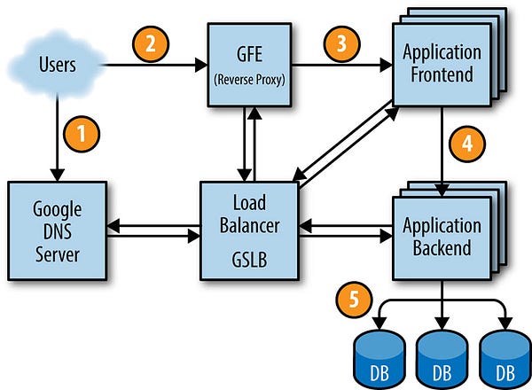
Figure 2–4 shows how a user’s request is serviced: first, the user points their browser to shakespeare.google.com. To obtain the corresponding IP address, the user’s device resolves the address with its DNS server (1). This request ultimately ends up at Google’s DNS server, which talks to GSLB. As GSLB keeps track of traffic load among frontend servers across regions, it picks which server IP address to send to this user.
This DNS load balancing is quite coarse, response times in 10s of minutes.
The browser connects to the HTTP server on this IP. This server (named the Google Frontend, or GFE) is a reverse proxy that terminates the TCP connection (2). The GFE looks up which service is required (web search, maps, or — in this case — Shakespeare). Again using GSLB, the server finds an available Shakespeare frontend server, and sends that server an RPC containing the HTTP request (3).
The response time on load reports is ≤10 seconds. Allowing traffic spikes to be handled extremely quickly.
It doesn’t matter if you have 10,000 servers, or just 10. We use GSLB to send the traffic to you. It just makes everything simpler to use the scalable infrastructure to get the requests to the right backend.
The load balancer will continuously check to see if the Application Frontend is running, responding to http, and reporting ‘healthy’. This means we can have a transient machine or server failure on any single backend, and route around failure.
The Shakespeare server analyzes the HTTP request and constructs a protobuf containing the word to look up. The Shakespeare frontend server now needs to contact the Shakespeare backend server: the frontend server contacts GSLB to obtain the BNS address of a suitable and unloaded backend server (4). That Shakespeare backend server now contacts a Bigtable server to obtain the requested data (5).
Everything using GSLB at every layer has an added benefit that hasn’t been covered yet: We can use our load balancer configuration to take any component of the system out of serving at any time. We call this ‘Draining’.
If a service is working fine globally, but has unusually high latency or errors in one datacenter, a first response action is to simply stop using that server in that datacenter temporarily. The traffic will simply flow to the closest available backends that can handle the capacity.
The answer is written to the reply protobuf and returned to the Shakespeare backend server. The backend hands a protobuf containing the results to the Shakespeare frontend server, which assembles the HTML and returns the answer to the user.
This entire chain of events is executed in the blink of an eye — just a few hundred milliseconds! Because many moving parts are involved, there are many potential points of failure; in particular, a failing GSLB would wreak havoc. However, Google’s policies of rigorous testing and careful rollout, in addition to our proactive error recovery methods such as graceful degradation, allow us to deliver the reliable service that our users have come to expect. After all, people regularly use www.google.com to check if their Internet connection is set up correctly.
I think this should be considerably faster than a few hundred milliseconds. Perhaps if everything was cold it might be a little slower.
Provided there are enough replicas of the server, and enough bigtable capacity: This architecture as stated could easily provide millions of queries per second.
Job and Data Organization
Load testing determined that our backend server can handle about 100 queries per second (QPS). Trials performed with a limited set of users lead us to expect a peak load of about 3,470 QPS, so we need at least 35 tasks. However, the following considerations mean that we need at least 37 tasks in the job, or N+2:
Google always says ‘QPS’ where others might say RPM/Requests per Minute or RPS/Requests per Second. This is a hangover from Google Search where we were measuring www.google.com search queries.
During updates, one task at a time will be unavailable, leaving 36 tasks.
A machine failure might occur during a task update, leaving only 35 tasks, just enough to serve peak load.
A closer examination of user traffic shows our peak usage is distributed globally: 1,430 QPS from North America, 290 from South America, 1,400 from Europe and Africa, and 350 from Asia and Australia. Instead of locating all backends at one site, we distribute them across the USA, South America, Europe, and Asia. Allowing for N+2 redundancy per region means that we end up with 17 tasks in the USA, 16 in Europe, and 6 in Asia. However, we decide to use 4 tasks (instead of 5) in South America, to lower the overhead of N+2 to N+1. In this case, we’re willing to tolerate a small risk of higher latency in exchange for lower hardware costs: if GSLB redirects traffic from one continent to another when our South American datacenter is over capacity, we can save 20% of the resources we’d spend on hardware. In the larger regions, we’ll spread tasks across two or three clusters for extra resiliency.
But actually what I do is spin up enough servers to handle global load, then I measure how much inter-continent traffic there is, and treat all regions separately and run enough capacity in each location to avoid ‘spilling’ across expensive links, and sanity-check that we can lose any region and serve all the traffic from other regions.
Because the backends need to contact the Bigtable holding the data, we need to also design this storage element strategically. A backend in Asia contacting a Bigtable in the USA adds a significant amount of latency, so we replicate the Bigtable in each region. Bigtable replication helps us in two ways: it provides resilience should a Bigtable server fail, and it lowers data-access latency. While Bigtable only offers eventual consistency, it isn’t a major problem because we don’t need to update the contents often.
Bigtable is just one of our storage technologies, but it’s easily the most scalable and appropriate ones for this use-case.
We’ve introduced a lot of terminology here; while you don’t need to remember it all, it’s useful for framing many of the other systems we’ll refer to later.原文链接:https://medium.com/@jerub/the-production-environment-at-google-part-2-610884268aaa