OpenGL.Tutorial16_ShadowMapping

ZC： 搜索了一下，bias只在 16_ShadowMapping.fragmentshader 中出现

ZC：

ZC：

1、Tutorial 16 _ Shadow mapping.html（http://www.opengl-tutorial.org/cn/intermediate-tutorials/tutorial-16-shadow-mapping/）

2、

在课程15中 我们学习了如何创建光照贴图，它包含静态光线。它生成了非常好的阴影，它无法处理动画模型。

阴影贴图是 当前的(到2016为止)创建动态阴影的方式。最好的事情就是 它们相当的容易去实现。糟糕的事情就是 很难是它正确的工作。

在本课程中，我们将介绍几本的算法，观察它的缺点，然后 采用一些技术来得到更好的结果。截止到写文章的时间(2012)  阴影贴图 依旧是一个沉重的研究课题，根据你的需要，我们将给你一些将来改善阴影贴图的方向。

In Tutorial 15 we learnt how to create lightmaps, which encompasses(包含) static lighting. While it produces very nice shadows, it doesn’t deal with animated(动画) models.

Shadow maps are the current (as of 2016) way to make dynamic shadows. The great thing about them is that it’s fairly(相当地) easy to get to work. The bad thing is that it’s terribly difficult to get to work right.

In this tutorial, we’ll first introduce the basic algorithm(算法), see its shortcomings(缺点), and then implement(执行;实施) some techniques(技术) to get better results. Since at time of writing (2012) shadow maps are still a heavily researched topic(研究课题), we’ll give you some directions to further improve(改善) your own shadowmap, depending on your needs.

Basic shadowmap

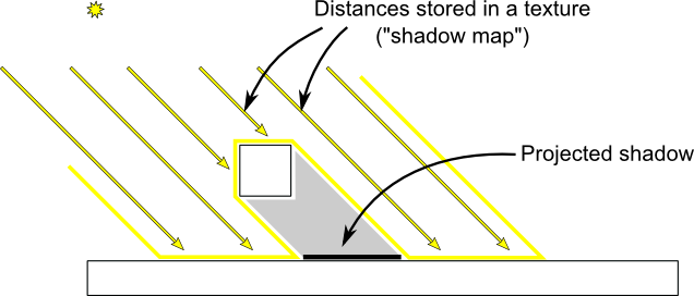
基本的 阴影贴图 算法包含 2个步骤。首先，场景 通过 光的视点。只有 每一个片段的深度是被计算的。（ZC：别的东西都不计算？） 第二步，场景照例渲染，但是 会有一个额外的检测 当前的片段是否是在阴影中。

"是否在阴影中"的测试 实际上很简单。如果当前的样本 比 阴影贴图的对应点 离光源更远的话，就说明 场景中 包含一个 更接近光源的物体。换句话说，当前的 片段 是位于阴影中。

下面的图，可能能够帮助你理解原理：

The basic shadowmap algorithm consists(包含) in two passes. First, the scene(场景) is rendered from the point of view of the light. Only the depth of each fragment is computed. Next, the scene is rendered as usual, but with an extra test to see it the current fragment is in the shadow.

The “being in the shadow” test is actually quite simple. If the current sample is further from the light than the shadowmap at the same point, this means that the scene contains an object that is closer(更接近) to the light. In other words, the current fragment is in the shadow.

The following image might help you understand the principle(原理) :

　　

Rendering the shadow map

在本教程中，我们只考虑定向的光源 - 光源是很远很远的 因此 我们可以认为所有的光线都是平行的。基于前面的这个想法，渲染阴影贴图 是使用正交投影矩阵(无近大远小) 来处理的。正交投影矩阵 与 平常的透视投影矩阵 类似，区别为 没有考虑透视效果 - 一个物体 不管它离 camera 是近还是远 看起来都将是一样的。

In this tutorial, we’ll only consider(考虑) directional(定向的) lights - lights that are so far away that all the light rays can be considered parallel(平行的). As such, rendering the shadow map is done with an orthographic(正交) projection matrix. An orthographic matrix is just like a usual perspective(透视的) projection matrix, except that no perspective is taken into account - an object will look the same whether it’s far or near the camera.

ZC：透视投影（Perspective Projection）与正射投影(Orthographic Projection) （https://blog.csdn.net/u011153817/article/details/52044722）

ZC：前者有 近大远小，　　　　　　　　后者没 近大远小。

Setting up the rendertarget and the MVP matrix

学习过教程第14课后，我们知道如何通过纹理渲染场景 以便后面通过着色器来访问它。

这里我们使用 1024x1024的 深度为16-bit 的纹理 来包含 阴影贴图。16位（深度） 用于阴影贴图 通常已经足够了。你可以自己随意的修改(实验;尝试)这些取值。注意我们使用深度纹理，并不是使用 深度渲染缓冲，∵ 我们后面要做取样操作。

Since Tutorial 14, you know how to render the scene into a texture in order to access it later from a shader.

Here we use a 1024x1024 16-bit depth texture to contain the shadow map. 16 bits are usually enough for a shadow map. Feel free to experiment(实验;尝试) with these values. Note that we use a depth texture, not a depth renderbuffer, since we’ll need to sample(取样) it later.

// The framebuffer, which regroups 0, 1, or more textures, and 0 or 1 depth buffer.
 GLuint FramebufferName = 0;
 glGenFramebuffers(1, &FramebufferName);// ZC: 该函数 在本课程中只调用了一次
 glBindFramebuffer(GL_FRAMEBUFFER, FramebufferName);// ZC: 搜索了一下，14课 和 16课 使用过此函数

 // Depth texture. Slower than a depth buffer, but you can sample it later in your shader
 GLuint depthTexture;
 glGenTextures(1, &depthTexture);// ZC: 该函数 在本课程中只调用了一次
 glBindTexture(GL_TEXTURE_2D, depthTexture);
 glTexImage2D(GL_TEXTURE_2D, 0,GL_DEPTH_COMPONENT16, 1024, 1024, 0,GL_DEPTH_COMPONENT, GL_FLOAT, 0);
 glTexParameteri(GL_TEXTURE_2D, GL_TEXTURE_MAG_FILTER, GL_NEAREST);
 glTexParameteri(GL_TEXTURE_2D, GL_TEXTURE_MIN_FILTER, GL_NEAREST);
 glTexParameteri(GL_TEXTURE_2D, GL_TEXTURE_WRAP_S, GL_CLAMP_TO_EDGE);
 glTexParameteri(GL_TEXTURE_2D, GL_TEXTURE_WRAP_T, GL_CLAMP_TO_EDGE);

 glFramebufferTexture(GL_FRAMEBUFFER, GL_DEPTH_ATTACHMENT, depthTexture, 0);

 glDrawBuffer(GL_NONE); // No color buffer is drawn to.

 // Always check that our framebuffer is ok
 if(glCheckFramebufferStatus(GL_FRAMEBUFFER) != GL_FRAMEBUFFER_COMPLETE)
 return false;

用光的视点来计算 MVP矩阵 然后渲染场景 的步骤如下：（ZC：下面这一段，现在还不太理解，以后再翻吧...）

• 投影矩阵 是 正射矩阵 

The MVP matrix used to render the scene from the light’s point of view is computed as follows :

• The Projection matrix is an orthographic matrix which will encompass(包围;围绕;围住) everything in the axis-aligned box (-10,10),(-10,10),(-10,20) on the X,Y and Z axes respectively. These values are made so that our entire *visible *scene is always visible ; more on this in the Going Further section.
• The View matrix rotates the world so that in camera space, the light direction is -Z (would you like to re-read Tutorial 3 ?)
• The Model matrix is whatever you want.

// ZC: 这是 光源照射的方向 的意思？
 glm::vec3 lightInvDir = glm::vec3(0.5f,2,2);

 // Compute the MVP matrix from the light's point of view
 glm::mat4 depthProjectionMatrix = glm::ortho<float>(-10,10,-10,10,-10,20);// ZC: 搜索了一下，这个函数在 第3课 和 第16课 使用
 glm::mat4 depthViewMatrix = glm::lookAt(lightInvDir, glm::vec3(0,0,0), glm::vec3(0,1,0));
 glm::mat4 depthModelMatrix = glm::mat4(1.0);
 glm::mat4 depthMVP = depthProjectionMatrix * depthViewMatrix * depthModelMatrix;

 // Send our transformation to the currently bound shader,
 // in the "MVP" uniform
 glUniformMatrix4fv(depthMatrixID, 1, GL_FALSE, &depthMVP[0][0])
// ZC: depthMVP对应的是 着色器文件中的 变量depthMVP（它只在 文件"16_DepthRTT.vertexshader"中出现）

The shaders

着色器的使用 在这个过程中 是非常简单的。顶点着色器 是一个传值的着色器，它 简单的计算顶点的齐次坐标位置。

The shaders used during this pass are very simple. The vertex shader is a pass-through shader which simply compute the vertex’ position in homogeneous coordinates(齐次坐标):

// ZC: 16_DepthRTT.vertexshader

#version 330 core

// Input vertex data, different for all executions of this shader.
layout(location = 0) in vec3 vertexPosition_modelspace;

// Values that stay constant for the whole mesh.
uniform mat4 depthMVP;

void main(){
 gl_Position =  depthMVP * vec4(vertexPosition_modelspace,1);
}

片段着色器 很简单：它只是简单的将片段深度信息写到 位置0 处（例如，在我们的深度纹理中）

The fragment shader is just as simple : it simply writes the depth of the fragment at location 0 (i.e. in our depth texture).

// ZC: 16_DepthRTT.fragmentshader

#version 330 core

// Ouput data
layout(location = 0) out float fragmentdepth;

void main(){
    // Not really needed, OpenGL does it anyway
    fragmentdepth = gl_FragCoord.z;
}

Result

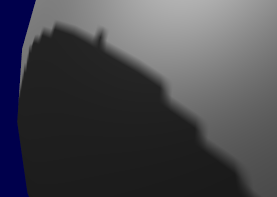
The resulting texture looks like this :

　　

暗的颜色表明是 小的z值；因此，墙的右上角 离camera 比较近。相对的，白色意味着z=1（齐次坐标），因此这回非常远。（ZC：是说 墙的右上角会离camera很远 的意思吗？）

A dark colour means a small z ; hence, the upper-right corner of the wall is near the camera. At the opposite, white means z=1 (in homogeneous coordinates), so this is very far.

Using the shadow map

Basic shader

现在我们回到我们的一般的着色器。我们计算每一个片段，我们必须测试它是否位于阴影贴图的"后面"。

要做这个工作的话，我们需要 在与创建阴影贴图的相同空间 计算当前片段的位置。（ZC：这里的空间是指类似如下的词?：模型空间->世界空间->摄像机空间->齐次坐标空间）。因此我们需要 用通常的MVP矩阵对它转换一次，再用深度MVP矩阵再转换一次。

一个小技巧。顶点位置 乘以 深度MVP矩阵 将得到 齐次坐标，值的范围为[-1,1]；但是纹理采样率必须在 [0,1]的范围。

例如，一个片段在屏幕中心的话 它的齐次坐标是(0,0)；但是 由于它要采样纹理的中心，UVs将会变成(0.5,0.5)。

这个现象 可以通过直接在片段着色器种调整提取坐标 来修正，但是 更有效的做法是 用下面的矩阵来乘这个齐次坐标，它简单的将坐标值除2（对角线：[-1,1]->-0.5,0.5）然后平移它们（下面的行：[-0.5,0.5]->[0,1]）

Now we go back to our usual shader. For each fragment that we compute, we must test whether it is “behind” the shadow map or not.

To do this, we need to compute the current fragment’s position in the same space that the one we used when creating the shadowmap. So we need to transform it once with the usual MVP matrix, and another time with the depthMVP matrix.

There is a little trick, though. Multiplying the vertex’ position by depthMVP will give homogeneous coordinates, which are in [-1,1] ; but texture sampling must be done in [0,1].

For instance, a fragment in the middle of the screen will be in (0,0) in homogeneous coordinates ; but since it will have to sample the middle of the texture, the UVs will have to be (0.5, 0.5).

This can be fixed by tweaking(调整) the fetch(提取) coordinates directly in the fragment shader but it’s more efficient to multiply the homogeneous coordinates by the following matrix, which simply divides(除法) coordinates by 2 ( the diagonal(对角线的) : [-1,1] -> [-0.5, 0.5] ) and translates them ( the lower row : [-0.5, 0.5] -> [0,1] ).

glm::mat4 biasMatrix(
0.5, 0.0, 0.0, 0.0,
0.0, 0.5, 0.0, 0.0,
0.0, 0.0, 0.5, 0.0,
0.5, 0.5, 0.5, 1.0
);
glm::mat4 depthBiasMVP = biasMatrix*depthMVP;

我们现在可以写我们的顶点着色器。它和之前的类似，只是 前面输出1个位置 而这里 输出2个位置 ：

• gl_Position 是 从当前camera 看到的顶点的位置
• ShadowCoord 是 上一次的camera 看到的顶点的位置（光源）

We can now write our vertex shader. It’s the same as before, but we output 2 positions instead of 1 :

• gl_Position is the position of the vertex as seen from the current camera
• ShadowCoord is the position of the vertex as seen from the last camera (the light)

// Output position of the vertex, in clip space : MVP * position
gl_Position =  MVP * vec4(vertexPosition_modelspace,1);

// Same, but with the light's view matrix
ShadowCoord = DepthBiasMVP * vec4(vertexPosition_modelspace,1);

片段着色器 将非常简单：

• texture( shadowMap, ShadowCoord.xy ).z 是 光源 和 最近的遮挡物 之间的距离
• ShadowCoord.z 是 光源 和 当前的片段 之间的距离

... 于是 如果当前的片段比最近的遮挡物远，就说明 我们位于阴影之中（是前面说到的最近的遮挡物造成的阴影）：

The fragment shader is then very simple :

• texture( shadowMap, ShadowCoord.xy ).z is the distance between the light and the nearest occluder(遮挡物)
• ShadowCoord.z is the distance between the light and the current fragment

… so if the current fragment is further than the nearest occluder, this means we are in the shadow (of said nearest occluder) :

float visibility = 1.0;
if ( texture( shadowMap, ShadowCoord.xy ).z  <  ShadowCoord.z){
    visibility = 0.5;
}

我们仅需要使用这个技术来修改我们的着色器。当然，周围环境的颜色没有修改，∵ 在它的生命周期里 它的目的是去伪造一些进来的光 即使当我们是处于阴影中（否则所有的失误将会是纯黑的）

We just have to use this knowledge to modify our shading. Of course, the ambient(周围环境的) colour isn’t modified, since its purpose in life is to fake(伪造) some incoming(进来的) light even when(即使当) we’re in the shadow (or everything would be pure black)

color =
 // Ambient : simulates indirect lighting
 MaterialAmbientColor +
 // Diffuse : "color" of the object
 visibility * MaterialDiffuseColor * LightColor * LightPower * cosTheta+
 // Specular : reflective highlight, like a mirror
 visibility * MaterialSpecularColor * LightColor * LightPower * pow(cosAlpha,5);

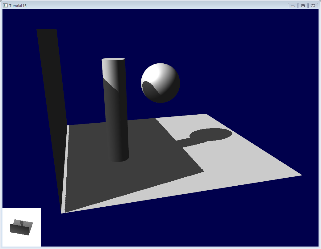
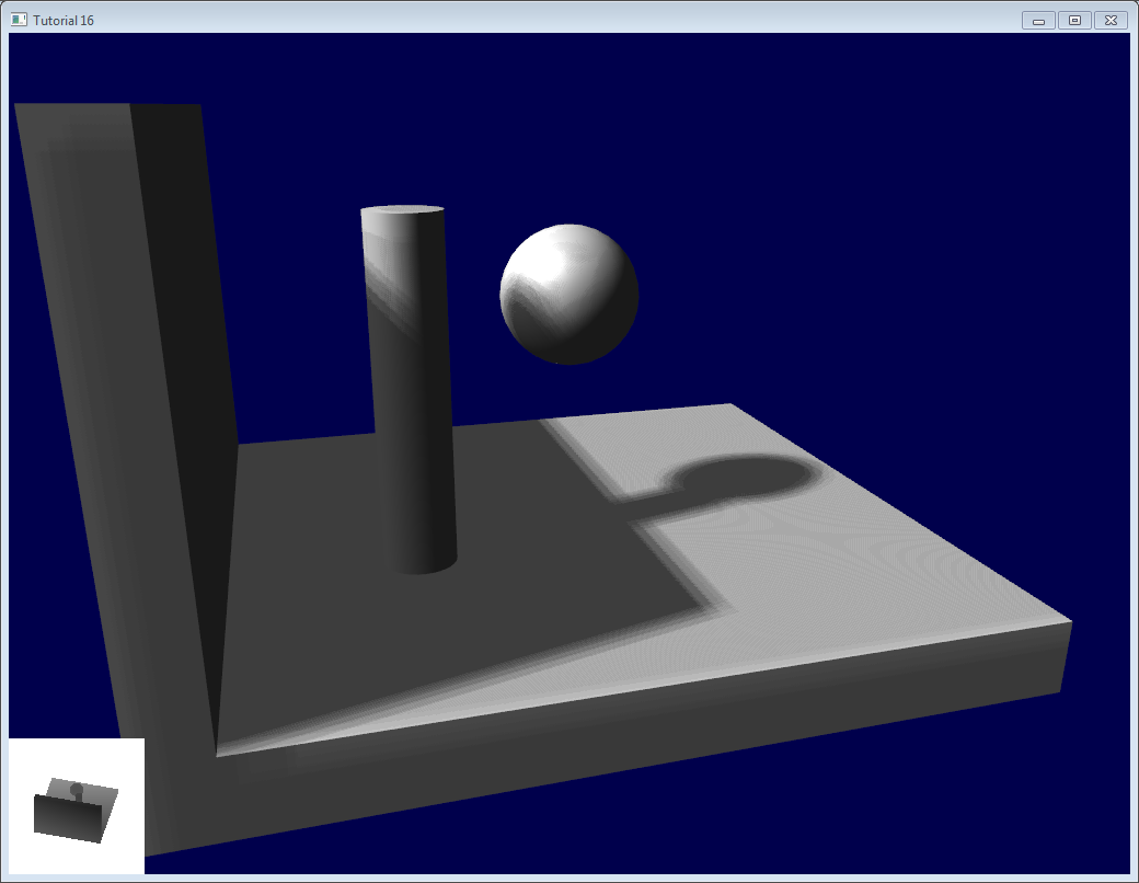
Result - Shadow acne(粉刺)

Here’s the result of the current code. Obviously, the global idea it there, but the quality is unacceptable.

　　

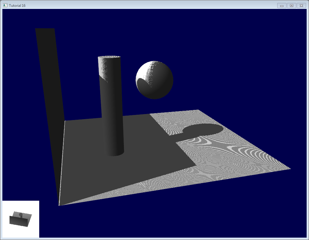
让我们观察图片中的每个问题。代码有两个方案：shadowmaps 和 shadowmaps_simple；开始不管哪个你最喜欢的。简单版的效果就像上面那样丑陋，但是 更容易理解。

Let’s look at each problem in this image. The code has 2 projects : shadowmaps and shadowmaps_simple; start with whichever(无论哪个) you like best. The simple version is just as ugly as the image above, but is simpler to understand.

Problems

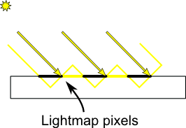
Shadow acne

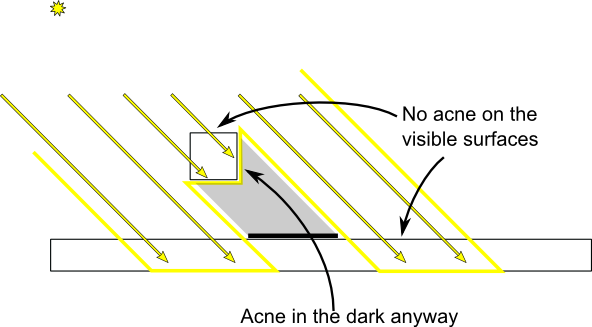
The most obvious problem is called shadow acne :

　　

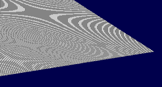
This phenomenon(现象) is easily explained with a simple image :

　　

此现象常用的"修复"方式是添加一个错误的白边：只有在 当前片段的深度（再次申明，是在光源空间） 真的是远离 光照贴图的值的时候 才会着色。我们添加一个偏移量 来达到效果：

The usual “fix” for this is to add an error margin(白边) : we only shade if the current fragment’s depth (again, in light space) is really far away from the lightmap value. We do this by adding a bias(偏见;偏心;偏向;偏爱;特殊能力;斜裁) :

float bias = 0.005;
float visibility = 1.0;
if ( texture( shadowMap, ShadowCoord.xy ).z  <  ShadowCoord.z-bias){　　// ZC: 搜索了一下，bias只在 16_ShadowMapping.fragmentshader 中出现
    visibility = 0.5;
}

The result is already much nicer :

　　

然而，你可能注意到了 由于我们设置的偏移量，在地面和墙面之间的工艺变得更差了。更重要的是，偏移量的值设置为0.005 看起来对于地面来说 太多了，但是 对于弯曲的表面来说 又显得不够：这种工艺在 圆柱和球 上 依然可见。

常见的方法是 根据倾斜角度值来修改偏移量：

However, you can notice that because of our bias, the artefact(人工制品，手工艺品) between the ground and the wall has gone worse. What’s more, a bias of 0.005 seems too much on the ground, but not enough on curved(弯曲) surface : some artefacts remain(仍然是;保持不变) on the cylinder(圆柱) and on the sphere(球).

A common approach(方法) is to modify the bias according to(根据) the slope(斜坡,倾斜) :

float bias = 0.005*tan(acos(cosTheta)); // cosTheta is dot( n,l ), clamped between 0 and 1
bias = clamp(bias, 0,0.01);

现在 即使在 弯曲表面上 Shadow acne 也不再出现了。

Shadow acne is now gone, even on curved surfaces.

　　

另一个技巧，这个技巧 可以依靠或不依靠几何学知识，它只通过阴影贴图来渲染背面。这会强制我们去使用特殊的厚墙几何学(见下一节内容"Peter Panning")，但是 至少acne是出现在阴影表面。（ZC：见下面的图，acne不会出现在 可视的表面，它只出现在阴影中的表面上(这个就无所谓了)）

Another trick(诡计;花招;骗局;把戏;), which may or may not work depending on(取决于) your geometry(几何学), is to render only the back faces in the shadow map. This forces us to have a special geometry ( see next section - Peter Panning ) with thick(厚的) walls, but at least, the acne(粉刺) will be on surfaces which are in the shadow :

　　

当渲染阴影贴图的时候，剔除正面的三角形：（ZC：看下面的代码，剔除正面的三角形，只画背面的三角形。[这是什么原理？为啥这样操作？]）

When rendering the shadow map, cull(剔除) front-facing(正面) triangles :

        // We don't use bias in the shader, but instead we draw back faces,
        // which are already separated from the front faces by a small distance
        // (if your geometry is made this way)
        glCullFace(GL_FRONT); // Cull front-facing triangles -> draw only back-facing triangles

然后，在渲染场景的时候，照常规方式渲染（背面渲染）

And when rendering the scene, render normally (backface culling)

         glCullFace(GL_BACK); // Cull back-facing triangles -> draw only front-facing triangles

除了使用偏移量之外，该方法（ZC：也）被用于代码中。

This method is used in the code, in addition to(另外，加之，除…之外(还)) the bias.

Peter Panning

现在 shadow acne 已经没有了，但是地面的着色仍然错误，这个错误使得墙看起来像是飞在空中（因此 把这个现象称为"Peter Panning"）。实际上，增加 偏移量反而会使情况更糟（ZC：这里是指 使用偏移量会使情况变更糟(不使用偏移量反而好一点)，还是说 增加偏移量的值的大小会使情况变得更糟(偏移量的取值小一点看起来更好)？）。

We have no shadow acne anymore, but we still have this wrong shading of the ground, making the wall to look as if it’s flying (hence(因此) the term(把…称为;把…叫做) “Peter Panning”). In fact, adding the bias made it worse.

　　

这问题很容易修正：不使用薄的集合图形。这样做有2个好处：

• 第一，它解决了"Peter Panning"问题：??????
• 第二，你可以在渲染光照贴图的时候打开背面剔除，∵ 现在，多边形的墙面对着墙，挡住了另一边，它不会使用背面剔除来渲染。

缺点就是 你需要渲染更多的三角形（2倍帧！）

This one is very easy to fix : simply avoid(避免) thin(薄的) geometry. This has two advantages(优势;优点) :

• First, it solves Peter Panning : it the geometry is more deep than your bias, you’re all set.
• Second, you can turn on backface culling when rendering the lightmap, because now, there is a polygon of the wall which is facing the light, which will occlude(使闭塞;堵塞) the other side, which wouldn’t be rendered with backface culling.

The drawback(缺点) is that you have more triangles to render ( two times per frame ! )

　　

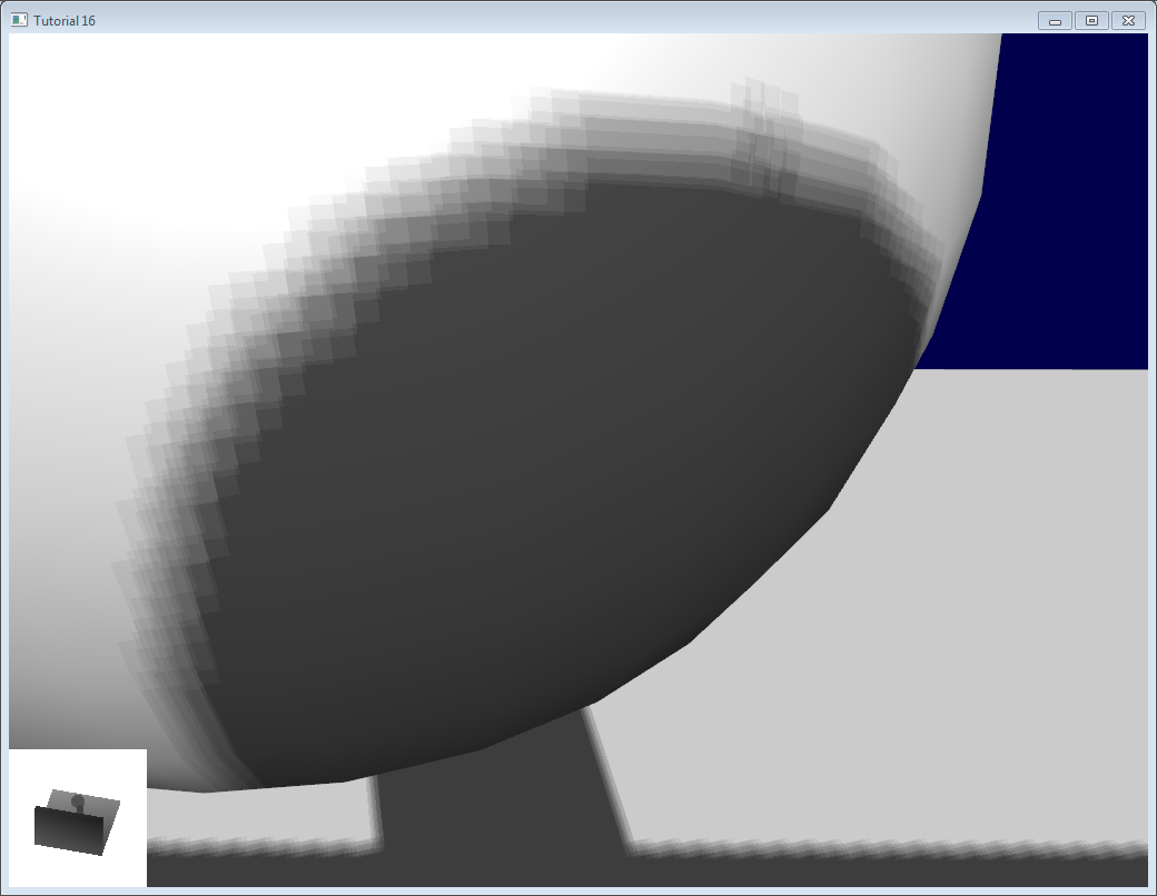
Aliasing(混叠;走样;混淆现象;混淆;别名问题)

即使使用了上面的2个技巧，你依然会发现在阴影边缘有走样的问题。换句话说，这一像素是白的，下一像素是黑的，在像素之间没有平滑的过渡。

Even with these two tricks, you’ll notice that there is still aliasing on the border of the shadow. In other words, one pixel is white, and the next is black, without a smooth transition(过渡) inbetween(中间).

　　

PCF

改善这个问题的最简单的方式是改变阴影贴图的采样类型 使用sampler2DShadow。结果就是你每次进行阴影贴图的采样，硬件实际上也会对临近的纹素也进行采样，把它们进行对比，使用双线性过滤比较结果 然后返回[0,1]的浮点数值。

例如，0.5表示2个采样在阴影中，2个采样在光照下。

注意，它不同于 单次过滤深度贴图采样！比较经常返回真或假；PCF返回 4个"真或假"的插值。

The easiest way to improve(改善) this is to change the shadowmap’s sampler type to sampler2DShadow. The consequence(结果) is that when you sample the shadowmap once, the hardware will in fact also sample the neighboring texels(纹素), do the comparison(比较) for all of them, and return a float in [0,1] with a bilinear(双线性的) filtering(过滤) of the comparison results.

For instance, 0.5 means that 2 samples are in the shadow, and 2 samples are in the light.

Note that it’s not the same than a single sampling of a filtered depth map ! A comparison always returns true or false; PCF gives a interpolation(插值) of 4 “true or false”.

　　

如你所见，阴影边缘变得光滑了，但是阴影贴图的纹素依然可见。

As you can see, shadow borders are smooth, but shadowmap’s texels are still visible.

Poisson Sampling

一个简单的方式解决这个问题 是使用N次采样来代替单次阴影贴图采样。结合PCF一起使用，将会得到非常好的结果，即使N值很小。这里是核心的4句代码：

An easy way to deal with this is to sample the shadowmap N times instead of once. Used in combination(结合) with PCF, this can give very good results, even with a small N. Here’s the code for 4 samples :

for (int i=0;i<4;i++){
  if ( texture( shadowMap, ShadowCoord.xy + poissonDisk[i]/700.0 ).z  <  ShadowCoord.z-bias ){
    visibility-=0.2;
  }
}

poissonDisk是一个常量数组，实例定义如下：

poissonDisk is a constant array defines for instance as follows :

vec2 poissonDisk[4] = vec2[](
  vec2( -0.94201624, -0.39906216 ),
  vec2( 0.94558609, -0.76890725 ),
  vec2( -0.094184101, -0.92938870 ),
  vec2( 0.34495938, 0.29387760 )
);

这样，根据你使用的采样次数的多少，生成的片段呈现深浅不一的阴影。

This way, depending on how many shadowmap samples will pass, the generated fragment will be more or less dark(阴影) :

　　

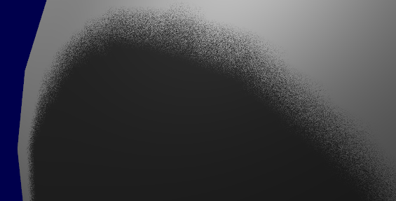
常量 700.0 指明了多少次的采样被“展开”。展开的太少，又会再次走样；展开的太多，将会导致这个结果：*带状（这个截屏没有使用PCF来得到激动人心的效果，而是使用16次采样来代替）*

The 700.0 constant defines how much the samples are “spread(展开;打开;摊开;使散开;张开;伸开)”. Spread them too little, and you’ll get aliasing(走样) again; too much, and you’ll get this :* banding (this screenshot doesn’t use PCF for a more dramatic(激动人心的) effect, but uses 16 samples instead) *

　　

　　

Stratified(分层的) Poisson Sampling

我们可以通过为每个像素选取不同的采样 来删除这个带状。这有2个主要的方法：分层的Poisson 或者 旋转的Poisson 。分层的方式选择不同的采样；旋转的方式使用相同的采样，但是会有一个随机的旋转 使得它们看起来不同。在本课程中我只讲解分层的版本。

与之前的版本唯一的不同点是  我们用随机的索引来为 poissonDisk 编索引：

We can remove this banding(带状) by choosing different samples for each pixel. There are two main methods : Stratified Poisson or Rotated Poisson. Stratified chooses different samples; Rotated always use the same, but with a random rotation so that they look different. In this tutorial I will only explain(解释) the stratified version.

The only difference with the previous version is that we index poissonDisk with a random index :

    for (int i=0;i<4;i++){
        int index = // A random number between 0 and 15, different for each pixel (and each i !)
        visibility -= 0.2*(1.0-texture( shadowMap, vec3(ShadowCoord.xy + poissonDisk[index]/700.0,  (ShadowCoord.z-bias)/ShadowCoord.w) ));
    }

We can generate a random number with a code like this, which returns a random number in [0,1] :

    float dot_product = dot(seed4, vec4(12.9898,78.233,45.164,94.673));
    return fract(sin(dot_product) * 43758.5453);

在我们的案例中，seed4 将会是 i(因此我们采样4个不同顶的位置)和...其它东西 的组合。我们可以使用 gl_FragCoord(像素在屏幕上的位置)，或 Position_worldspace：

In our case, seed4 will be the combination of i (so that we sample at 4 different locations) and … something else. We can use gl_FragCoord ( the pixel’s location on the screen ), or Position_worldspace :

        //  - A random sample, based on the pixel's screen location.
        //    No banding, but the shadow moves with the camera, which looks weird.
        int index = int(16.0*random(gl_FragCoord.xyy, i))%16;
        //  - A random sample, based on the pixel's position in world space.
        //    The position is rounded to the millimeter to avoid too much aliasing
        //int index = int(16.0*random(floor(Position_worldspace.xyz*1000.0), i))%16;

这会生成一个像上面图片消失的样板，视觉噪音的花费。仍然，好的噪音 比那些样式更讨厌。

This will make patterns(模式;方式;范例;典范;榜样;样板;图案;花样;式样) such as in the picture above disappear(消失;不见;), at the expense(开销;开支;花费) of visual(视力的;视觉的) noise. Still(仍然), a well-done(干得好的) noise is often less objectionable(令人不快的;令人反感的;讨厌的) than these patterns.

See tutorial16/ShadowMapping.fragmentshader for three example implementions.

Going further

即使有了这些技巧，我们的阴影还是有许多许多的地方可以改进。这些是最常见的：

Even with all these tricks, there are many, many ways in which our shadows could be improved. Here are the most common :

Early bailing

使用4次不同的采样 来替代 16次的采样。如果所有的(ZC：像素)都在光线中或在阴影中，你可能考虑 所有的16次采样都得到相同的结果：尽早保释。如果有些不同，你可能在阴影的边缘，于是 16次采样时必须的。

Instead of taking 16 samples for each fragment (again, it’s a lot), take 4 distant(遥远的;远处的;久远的;不相似的;不同的;远亲的;远房的) samples. If all of them are in the light or in the shadow, you can probably consider that all 16 samples would have given the same result : bail（允许保释(某人);(尤指迅速地)离开;与…搭讪(常指对方不愿意)） early. If some are different, you’re probably on a shadow boundary, so the 16 samples are needed.

Spot(斑点;污迹;) lights

处理光斑需要一些不同的改变。最明显的一点就是 用 透视投影矩阵 来替换 正射投影矩阵。

Dealing with spot lights requires very few changes. The most obvious(明显的) one is to change the orthographic(正射) projection matrix into a perspective projection matrix :

glm::vec3 lightPos(5, 20, 20);
glm::mat4 depthProjectionMatrix = glm::perspective<float>(glm::radians(45.0f), 1.0f, 2.0f, 50.0f);
glm::mat4 depthViewMatrix = glm::lookAt(lightPos, lightPos-lightInvDir, glm::vec3(0,1,0));

同样的，用正射投影替代透视投影。使用 texture2Dproj 来解释 透视分割（见 课程4-矩阵 里的 footnotes）。ZC：课程3 才是讲 矩阵 的.. 而且 没找到 哪个课程里有 footnotes节的内容... ZC：footnotes（脚注）

第二步是把 透视 引入到着色器中。（见 课程4 footnotes节。在 坚果壳中，透视投影矩阵 实际上没有任何透视的作用。它在硬件中被完成，通过用w来分割投影坐标。这里，我们在着色器中模拟转换，于是我们需要自己做投影分割。顺便一提，正射矩阵 常常生成 齐次的向量 w=1，这就是它不会有透视效果的原因）

这里有两个方式可以在GLSL中采用。第二个方式使用内置的 textureProj 函数，但是 2个方法产生完全相同的效果。

same thing, but with a perspective(透视) frustum(截锥体) instead of an orthographic frustum. Use texture2Dproj to account for perspective-divide(透视分割) (see footnotes in tutorial 4 - Matrices)

The second step is to take into account(考虑到;把…计算在内) the perspective in the shader. (see footnotes in tutorial 4 - Matrices. In a nutshell(坚果壳), a perspective projection matrix actually doesn’t do any perspective at all. This is done by the hardware, by dividing the projected coordinates by w. Here, we emulate(仿真;模仿) the transformation in the shader, so we have to do the perspective-divide ourselves. By the way, an orthographic matrix always generates homogeneous(同种类的) vectors with w=1, which is why they don’t produce(生产;制造;生长;出产;) any perspective)

Here are two way(双向;双向的;) to do this in GLSL. The second uses the built-in(内置的) textureProj function, but both methods produce exactly the same result.

if ( texture( shadowMap, (ShadowCoord.xy/ShadowCoord.w) ).z  <  (ShadowCoord.z-bias)/ShadowCoord.w )
if ( textureProj( shadowMap, ShadowCoord.xyw ).z  <  (ShadowCoord.z-bias)/ShadowCoord.w )

Point lights

相同的，但是使用深度立体映射。立体映射是一个6纹理的集合，立体的每一面对应一个；更重要的是，它不是访问标准的UV坐标，而是一个3D向量所代表的方向。

深度储存在空间的所有方向中，这使得 阴影投射到光点的四面八方变得可行。

Same thing, but with depth cubemaps. A cubemap is a set of 6 textures, one on each side of a cube; what’s more(更重要的是), it is not accessed(访问，存取) with standard UV coordinates, but with a 3D vector representing(代表) a direction.

The depth is stored for all directions in space, which make possible for shadows to be cast(投射) all around(四面八方) the point light.

Combination of several lights（ZC：组合多光源？）

算法可以处理多个光源，但是 牢记一点 每个光源为了产生阴影贴入都需要额外的场景渲染。当使用阴影时 将需要 巨大数量的内存，可能一会就内存不足了。

The algorithm(算法) handles several lights, but keep in mind(牢记) that each light requires an additional rendering of the scene in order to(为了) produce the shadowmap. This will require an enormous(巨大的) amount of memory when applying(使用;应用;) the shadows, and you might become bandwidth-limited(带宽有限) very quickly.

Automatic light frustum(截锥体)

在本课程中，光的截锥体 认为的设置 包含整个场景。当它工作在受限制的例子中时，它将被避免。如果你映射 1Km * 1Km，1024*1024的阴影贴图 中的 每个图素 将占用 1平方米；这是 无说服力的。光源的投影矩阵 应该是 尽可能的紧。

至于光斑，能通过调整它的范围来很方便的改变。

定向光源，像太阳，更难处理：它们是真的照亮了整个场景。这里有一个方法来计算光截锥体：

1. 潜在的阴影接收者，简写为PSRs，是 同时属于光截锥体的物体，对于视角截锥体，对于场景边界盒。对于它们名字的建议，这些物体是可以被阴影化的：它们对于相机和光源来说是 可见的。
   
2. 潜在的阴影角轮，或 简称为 PCFs，是所有的 潜在阴影接收者，加上 介于它们和光源之间的物体（物体可能不可见单是仍然投射可视的阴影）

因此，计算 光投影矩阵，呈现所有可视的物体，删除那些太远的物体，计算它们的边界盒子；添加介于边界盒和光源之间的物体，然后计算新的边界盒（但是这一次，沿光的方向对齐）

精确的

In this tutorial, the light frustum hand-crafted(手工的;) to contain(包含) the whole scene. While this works in this restricted(受限制的) example, it should be avoided(避免). If your map is 1Km x 1Km, each texel(图素;纹元;) of your 1024x1024 shadowmap will take 1 square meter; this is lame(站不住脚的;无说服力的). The projection matrix of the light should be(应该是) as tight(紧的) as possible.

For spot lights, this can be easily changed by tweaking(调整) its range.

Directional(指向性;定向;方向性;平行光;方向的) lights, like the sun, are more tricky(难办的;难对付的;狡猾的;诡计多端的) : they really do illuminate(照亮) the whole scene. Here’s a way to compute a the light frustum :

1. Potential(潜在的;可能的) Shadow Receivers, or PSRs for short, are objects which belong at the same time to(同时属于) the light frustum, to the view frustum, and to the scene bounding box. As their name suggest(建议), these objects are susceptible(易受影响(或伤害等);敏感;可能…的;可以…的) to be shadowed : they are visible by the camera and by the light.

2. Potential Shadow Casters(调味瓶;角轮;万向轮;小脚轮), or PCFs, are all the Potential Shadow Receivers, plus all objects which lie between them and the light (an object may not be visible but still cast(投射) a visible shadow).

So, to compute the light projection matrix, take all visible objects, remove those which are too far away, and compute their bounding box; Add the objects which lie(躺) between this bounding box and the light, and compute the new bounding box (but this time, aligned(排整齐; 校准;) along the light direction).

Precise(精确的) computation of these sets involve(包含) computing convex(凸面的) hulls(船身;船体) intersections(交点;横断;交叉;相交), but this method is much easier to implement.

This method will result in popping(发爆裂声;) when objects disappear from the frustum, because the shadowmap resolution(分辨率) will suddenly increase(增加). Cascaded(级联的) Shadow Maps don’t have this problem, but are harder to implement, and you can still compensate(补偿) by smoothing the values over time(随着时间的推移；超时).

Exponential(指数函数;指数分布;指数的) shadow maps

Exponential shadow maps try to limit aliasing(混叠) by assuming(假设) that a fragment which is in the shadow, but near the light surface, is in fact “somewhere in the middle”. This is related to the bias, except that the test isn’t binary(二元的) anymore : the fragment gets darker and darker when its distance to the lit surface increases.

This is cheating, obviously, and artefacts(人工制品) can appear when two objects overlap(重叠).

Light-space perspective Shadow Maps

LiSPSM tweaks(调整) the light projection matrix in order to get more precision(精度) near the camera. This is especially(尤其;特别;) important in case of “duelling(使（另一人）参加决斗;反对;参加正式决斗) frustra(徒劳的；无效的；无理的；错误的)” : you look in a direction, but a spot light “looks” in the opposite direction. You have a lot of shadowmap precision(精度) near the light, i.e. far from you, and a low resolution(分辨率) near the camera, where you need it the most.

However LiSPM is tricky to implement. See the references for details on the implementation.

Cascaded(级联的;串联的;串接;级联式) shadow maps

CSM deals with the exact same problem than LiSPSM, but in a different way. It simply uses several (2-4) standard shadow maps for different parts of the view frustum. The first one deals with the first meters, so you’ll get great resolution for a quite little zone. The next shadowmap deals with more distant(远的) objects. The last shadowmap deals with a big part of the scene, but due tu the perspective, it won’t be more visually important than the nearest zone.

Cascarded shadow maps have, at time of writing (2012), the best complexity/quality ratio. This is the solution of choice in many cases.

Conclusion(结论)

As you can see, shadowmaps are a complex subject. Every year, new variations and improvement are published, and to day, no solution is perfect.

Fortunately, most of the presented methods can be mixed together : It’s perfectly possible to have Cascaded Shadow Maps in Light-space Perspective, smoothed with PCF… Try experimenting with all these techniques.

As a conclusion, I’d suggest you to stick to pre-computed lightmaps whenever possible, and to use shadowmaps only for dynamic objects. And make sure that the visual quality of both are equivalent : it’s not good to have a perfect static environment and ugly dynamic shadows, either.

3、glm::mat4 ?? = glm::ortho<float>( T left, T right, T bottom, T top, T zNear, T zFar ); 相关资料：

　　OpenGL坐标系统 - Terrell - 博客园.html（https://www.cnblogs.com/tandier/p/8110977.html）
　　Opengl中矩阵和perspective_ortho的相互转换 - BIT祝威 - 博客园.html（https://www.cnblogs.com/bitzhuwei/p/4733264.html）
　　OpenGL学习笔记(4) GLM库的使用 - haowenlai2008的博客 - CSDN博客.html（https://blog.csdn.net/haowenlai2008/article/details/88853263）
　　4.opengl编程第二步：设置平截头体和输出空间 - 简书.html（https://www.jianshu.com/p/417c52a07cd4）

4、Shadow acne 相关资料：

　　Unity基础(5) Shadow Map 概述 - 细雨淅淅 - 博客园.html（https://www.cnblogs.com/zsb517/p/6696652.html）

　　　　关于Shadow Mapping产生的Shadow Acne，我的理解是不是有问题？ - 知乎.html（https://www.zhihu.com/question/49090321）

5、