(批量)梯度下降法
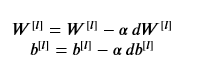


 1 import numpy as np
 2 import matplotlib.pyplot as plt
 3 import scipy.io
 4 import math
 5 import sklearn
 6 import sklearn.datasets
 7
 8 from opt_utils import load_params_and_grads, initialize_parameters, forward_propagation, backward_propagation
 9 from opt_utils import compute_cost, predict, predict_dec, plot_decision_boundary, load_dataset
10 from testCases_v3 import *
11
12 # %matplotlib inline
13 plt.rcParams['figure.figsize'] = (7.0, 4.0) # set default size of plots
14 plt.rcParams['image.interpolation'] = 'nearest'
15 plt.rcParams['image.cmap'] = 'gray'
16
17
18 # GRADED FUNCTION: update_parameters_with_gd
19 def update_parameters_with_gd(parameters, grads, learning_rate):
20     """
21     Update parameters using one step of gradient descent
22
23     Arguments:
24     parameters -- python dictionary containing your parameters to be updated:
25                     parameters['W' + str(l)] = Wl
26                     parameters['b' + str(l)] = bl
27     grads -- python dictionary containing your gradients to update each parameters:
28                     grads['dW' + str(l)] = dWl
29                     grads['db' + str(l)] = dbl
30     learning_rate -- the learning rate, scalar.
31
32     Returns:
33     parameters -- python dictionary containing your updated parameters
34     """
35
36     L = len(parameters) // 2 # number of layers in the neural networks
37
38     # Update rule for each parameter
39     for l in range(L):
40         ### START CODE HERE ### (approx. 2 lines)
41         parameters['W'+str(l+1)]=parameters['W'+str(l+1)]-learning_rate*grads['dW'+str(l+1)]
42         parameters['b'+str(l+1)]=parameters['b'+str(l+1)]-learning_rate*grads['db'+str(l+1)]
43         ### END CODE HERE ###
44
45     return parameters
批量梯度下降(mini-batch size=m)
随机梯度下降(mini-batch size=1)
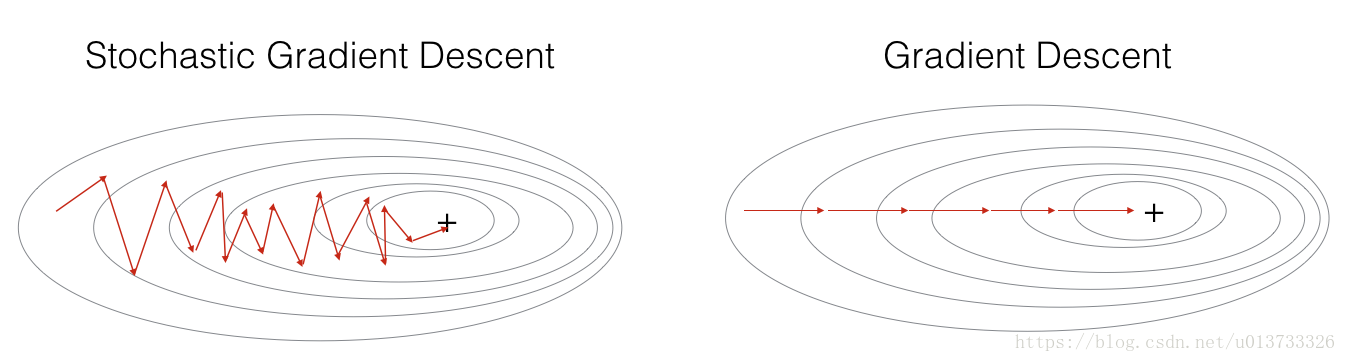
 1 #(Batch) Gradient Descent:
 2 X = data_input
 3 Y = labels
 4 parameters = initialize_parameters(layers_dims)
 5 for i in range(0, num_iterations):
 6     # Forward propagation
 7     a, caches = forward_propagation(X, parameters)
 8     # Compute cost.
 9     cost = compute_cost(a, Y)
10     # Backward propagation.
11     grads = backward_propagation(a, caches, parameters)
12     # Update parameters.
13     parameters = update_parameters(parameters, grads)
14
15 #Stochastic Gradient Descent:
16 X = data_input
17 Y = labels
18 parameters = initialize_parameters(layers_dims)
19 for i in range(0, num_iterations):
20     for j in range(0, m):
21         # Forward propagation
22         a, caches = forward_propagation(X[:,j], parameters)
23         # Compute cost
24         cost = compute_cost(a, Y[:,j])
25         # Backward propagation
26         grads = backward_propagation(a, caches, parameters)
27         # Update parameters.
28         parameters = update_parameters(parameters, grads)
mini-batch梯度下降
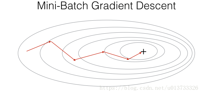
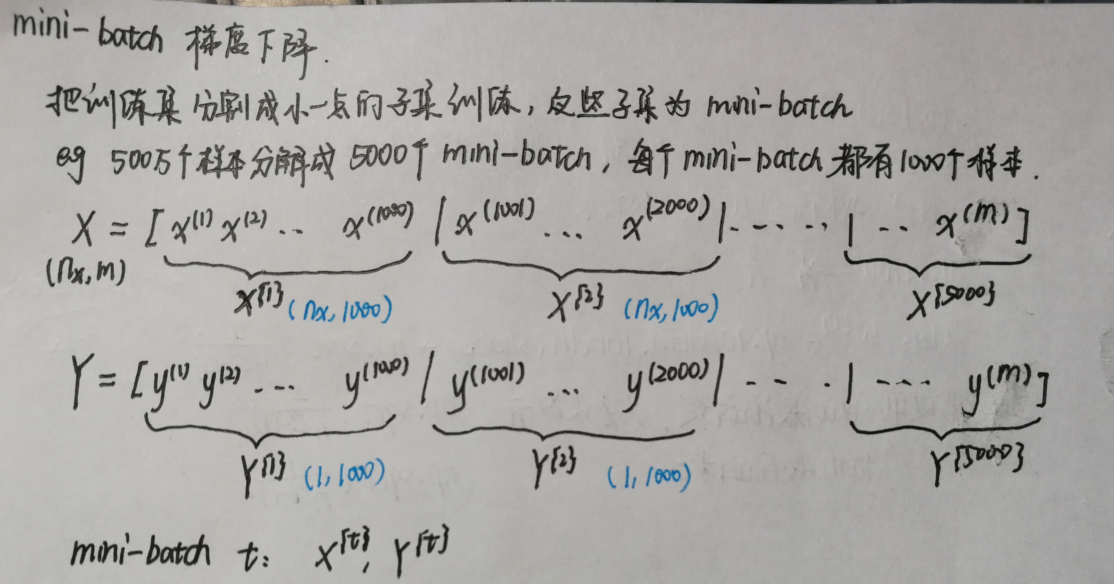
图中直接按训练集的原顺序分割,代码中先使用permutation函数打乱后再分割。
 1 def random_mini_batches(X, Y, mini_batch_size = 64, seed = 0):
 2     """
 3     Creates a list of random minibatches from (X, Y)
 4
 5     Arguments:
 6     X -- input data, of shape (input size, number of examples)
 7     Y -- true "label" vector (1 for blue dot / 0 for red dot), of shape (1, number of examples)
 8     mini_batch_size -- size of the mini-batches, integer
 9
10     Returns:
11     mini_batches -- list of synchronous (mini_batch_X, mini_batch_Y)
12     """
13
14     np.random.seed(seed)            # To make your "random" minibatches the same as ours
15     m = X.shape[1]                  # number of training examples
16     mini_batches = []
17
18     # Step 1: Shuffle (X, Y)
19     permutation = list(np.random.permutation(m))
20     shuffled_X = X[:, permutation]
21     shuffled_Y = Y[:, permutation].reshape((1,m))
22
23     # Step 2: Partition (shuffled_X, shuffled_Y). Minus the end case.
24     num_complete_minibatches = math.floor(m/mini_batch_size) # number of mini batches of size mini_batch_size in your partitionning
25     for k in range(0, num_complete_minibatches):
26         ### START CODE HERE ### (approx. 2 lines)
27         mini_batch_X=shuffled_X[:,k*mini_batch_size:(k+1)*mini_batch_size]
28         mini_batch_Y=shuffled_Y[:,k*mini_batch_size:(k+1)*mini_batch_size]
29         ### END CODE HERE ###
30
31         mini_batch = (mini_batch_X, mini_batch_Y)
32         mini_batches.append(mini_batch)
33
34     # Handling the end case (last mini-batch < mini_batch_size)
35     if m % mini_batch_size != 0:
36         ### START CODE HERE ### (approx. 2 lines)
37         mini_batch_X=shuffled_X[:,mini_batch_size * num_complete_minibatches:]
38         mini_batch_Y=shuffled_Y[:,mini_batch_size * num_complete_minibatches:]
39         ### END CODE HERE ###
40
41         mini_batch = (mini_batch_X, mini_batch_Y)
42         mini_batches.append(mini_batch)
43
44     return mini_batches
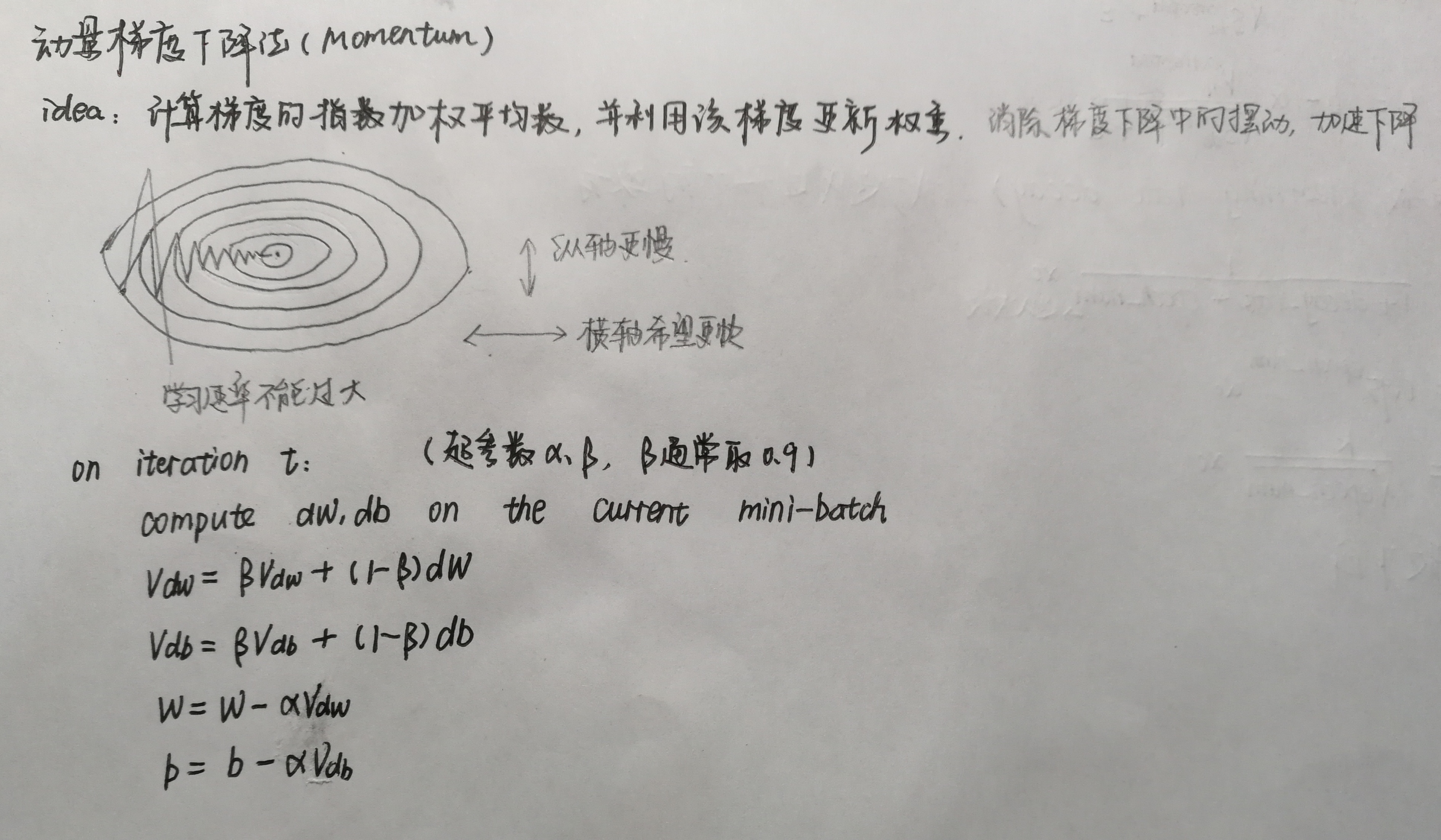
动量梯度下降法
初始化参数
 1 def initialize_velocity(parameters):
 2     """
 3     Initializes the velocity as a python dictionary with:
 4                 - keys: "dW1", "db1", ..., "dWL", "dbL"
 5                 - values: numpy arrays of zeros of the same shape as the corresponding gradients/parameters.
 6     Arguments:
 7     parameters -- python dictionary containing your parameters.
 8                     parameters['W' + str(l)] = Wl
 9                     parameters['b' + str(l)] = bl
10
11     Returns:
12     v -- python dictionary containing the current velocity.
13                     v['dW' + str(l)] = velocity of dWl
14                     v['db' + str(l)] = velocity of dbl
15     """
16
17     L = len(parameters) // 2 # number of layers in the neural networks
18     v = {}
19
20     # Initialize velocity
21     for l in range(L):
22         ### START CODE HERE ### (approx. 2 lines)
23         v['dW'+str(l+1)]=np.zeros_like(parameters['W'+str(l+1)])
24         v['db'+str(l+1)]=np.zeros_like(parameters['b'+str(l+1)])
25         ### END CODE HERE ###
26
27     return v
更新参数
 1 def update_parameters_with_momentum(parameters, grads, v, beta, learning_rate):
 2     """
 3     Update parameters using Momentum
 4
 5     Arguments:
 6     parameters -- python dictionary containing your parameters:
 7                     parameters['W' + str(l)] = Wl
 8                     parameters['b' + str(l)] = bl
 9     grads -- python dictionary containing your gradients for each parameters:
10                     grads['dW' + str(l)] = dWl
11                     grads['db' + str(l)] = dbl
12     v -- python dictionary containing the current velocity:
13                     v['dW' + str(l)] = ...
14                     v['db' + str(l)] = ...
15     beta -- the momentum hyperparameter, scalar
16     learning_rate -- the learning rate, scalar
17
18     Returns:
19     parameters -- python dictionary containing your updated parameters
20     v -- python dictionary containing your updated velocities
21     """
22
23     L = len(parameters) // 2 # number of layers in the neural networks
24
25     # Momentum update for each parameter
26     for l in range(L):
27
28         ### START CODE HERE ### (approx. 4 lines)
29         # compute velocities
30         v["dW" + str(l + 1)] = beta * v["dW" + str(l + 1)] + (1 - beta) * grads['dW' + str(l + 1)]
31         v["db" + str(l + 1)] = beta * v["db" + str(l + 1)] + (1 - beta) * grads['db' + str(l + 1)]
32         # update parameters
33         parameters["W" + str(l + 1)] = parameters["W" + str(l + 1)] - learning_rate * v["dW" + str(l + 1)]
34         parameters["b" + str(l + 1)] = parameters["b" + str(l + 1)] - learning_rate * v["db" + str(l + 1)]
35         ### END CODE HERE ###
36
37     return parameters, v
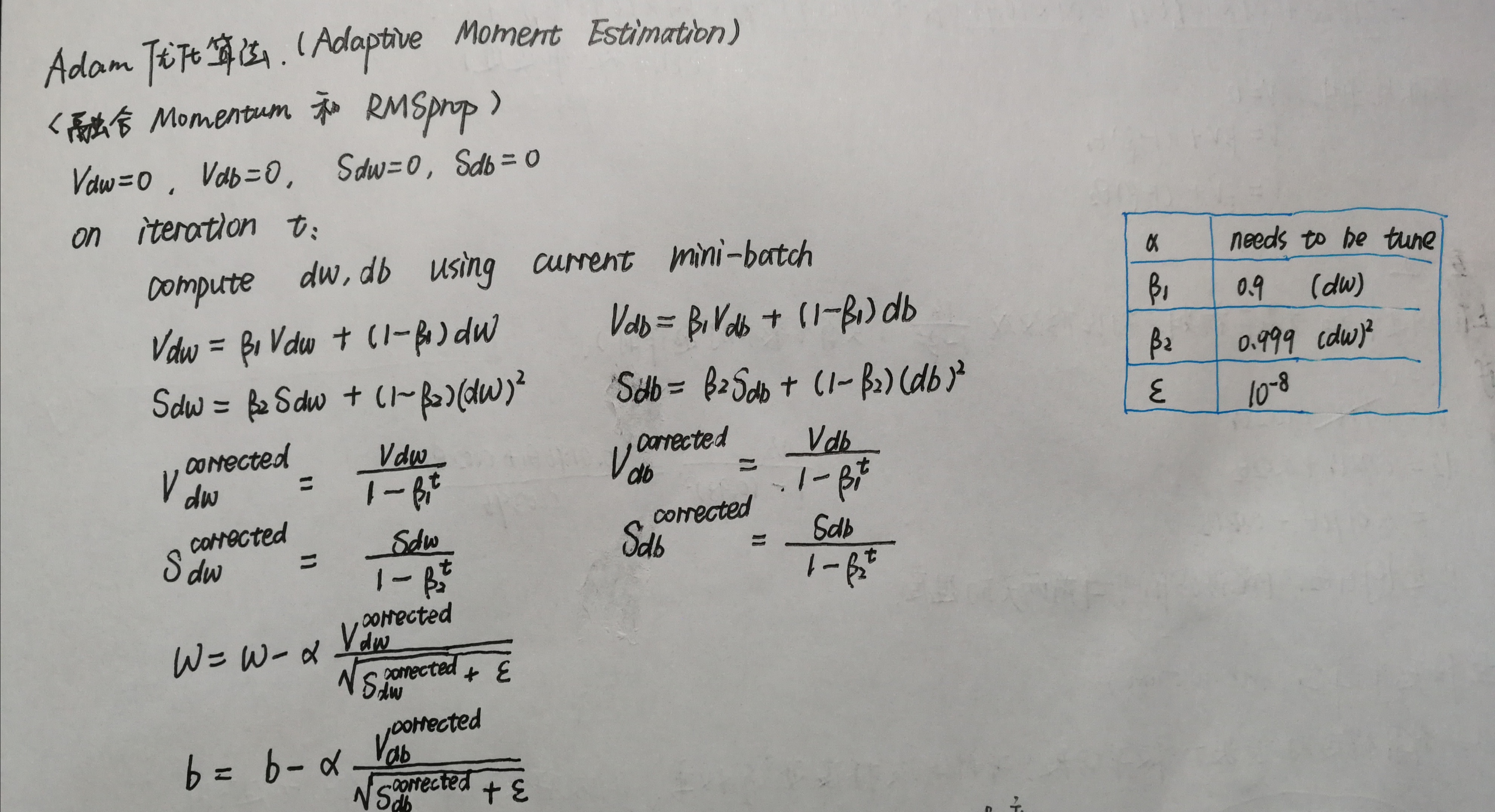
Adam优化算法
初始化参数
 1 def initialize_adam(parameters) :
 2     """
 3     Initializes v and s as two python dictionaries with:
 4                 - keys: "dW1", "db1", ..., "dWL", "dbL"
 5                 - values: numpy arrays of zeros of the same shape as the corresponding gradients/parameters.
 6
 7     Arguments:
 8     parameters -- python dictionary containing your parameters.
 9                     parameters["W" + str(l)] = Wl
10                     parameters["b" + str(l)] = bl
11
12     Returns:
13     v -- python dictionary that will contain the exponentially weighted average of the gradient.
14                     v["dW" + str(l)] = ...
15                     v["db" + str(l)] = ...
16     s -- python dictionary that will contain the exponentially weighted average of the squared gradient.
17                     s["dW" + str(l)] = ...
18                     s["db" + str(l)] = ...
19
20     """
21
22     L = len(parameters) // 2 # number of layers in the neural networks
23     v = {}
24     s = {}
25
26     # Initialize v, s. Input: "parameters". Outputs: "v, s".
27     for l in range(L):
28     ### START CODE HERE ### (approx. 4 lines)
29         v["dW" + str(l+1)] = np.zeros_like(parameters['W'+str(l+1)])
30         v["db" + str(l+1)] = np.zeros_like(parameters['b'+str(l+1)])
31
32         s["dW" + str(l+1)] = np.zeros_like(parameters['W'+str(l+1)])
33         s["db" + str(l+1)] = np.zeros_like(parameters['b'+str(l+1)])
34     ### END CODE HERE ###
35
36     return v, s
更新参数
 1 def update_parameters_with_adam(parameters, grads, v, s, t, learning_rate=0.01,
 2                                 beta1=0.9, beta2=0.999, epsilon=1e-8):
 3     """
 4     Update parameters using Adam
 5
 6     Arguments:
 7     parameters -- python dictionary containing your parameters:
 8                     parameters['W' + str(l)] = Wl
 9                     parameters['b' + str(l)] = bl
10     grads -- python dictionary containing your gradients for each parameters:
11                     grads['dW' + str(l)] = dWl
12                     grads['db' + str(l)] = dbl
13     v -- Adam variable, moving average of the first gradient, python dictionary
14     s -- Adam variable, moving average of the squared gradient, python dictionary
15     learning_rate -- the learning rate, scalar.
16     beta1 -- Exponential decay hyperparameter for the first moment estimates
17     beta2 -- Exponential decay hyperparameter for the second moment estimates
18     epsilon -- hyperparameter preventing division by zero in Adam updates
19
20     Returns:
21     parameters -- python dictionary containing your updated parameters
22     v -- Adam variable, moving average of the first gradient, python dictionary
23     s -- Adam variable, moving average of the squared gradient, python dictionary
24     """
25
26     L = len(parameters) // 2                 # number of layers in the neural networks
27     v_corrected = {}                         # Initializing first moment estimate, python dictionary
28     s_corrected = {}                         # Initializing second moment estimate, python dictionary
29
30     # Perform Adam update on all parameters
31     for l in range(L):
32         # Moving average of the gradients. Inputs: "v, grads, beta1". Output: "v".
33         ### START CODE HERE ### (approx. 2 lines)
34         v['dW'+str(l+1)]=beta1*v["dW"+str(l+1)]+(1-beta1)*grads['dW'+str(l+1)]
35         v['db'+str(l+1)]=beta1*v["db"+str(l+1)]+(1-beta1)*grads['db'+str(l+1)]
36         ### END CODE HERE ###
37
38         # Compute bias-corrected first moment estimate. Inputs: "v, beta1, t". Output: "v_corrected".
39         ### START CODE HERE ### (approx. 2 lines)
40         v_corrected['dW'+str(l+1)]=v['dW'+str(l+1)]/(1-beta1**t)
41         v_corrected['db'+str(l+1)]=v['db'+str(l+1)]/(1-beta1**t)
42         ### END CODE HERE ###
43
44         # Moving average of the squared gradients. Inputs: "s, grads, beta2". Output: "s".
45         ### START CODE HERE ### (approx. 2 lines)
46         s['dW'+str(l+1)]=beta2*s["dW"+str(l+1)]+(1-beta2)*(grads['dW'+str(l+1)])**2
47         s['db'+str(l+1)]=beta2*s["db"+str(l+1)]+(1-beta2)*(grads['db'+str(l+1)])**2
48         ### END CODE HERE ###
49
50         # Compute bias-corrected second raw moment estimate. Inputs: "s, beta2, t". Output: "s_corrected".
51         ### START CODE HERE ### (approx. 2 lines)
52         s_corrected['dW'+str(l+1)]=s['dW'+str(l+1)]/(1-beta2**t)
53         s_corrected['db'+str(l+1)]=s['db'+str(l+1)]/(1-beta2**t)
54         ### END CODE HERE ###
55
56         # Update parameters. Inputs: "parameters, learning_rate, v_corrected, s_corrected, epsilon". Output: "parameters".
57         ### START CODE HERE ### (approx. 2 lines)
58         parameters['W'+str(l+1)]=parameters['W'+str(l+1)]-learning_rate*(v_corrected['dW'+str(l+1)]/np.sqrt(s_corrected['dW'+str(l+1)]+epsilon))
59         parameters['b'+str(l+1)]=parameters['b'+str(l+1)]-learning_rate*(v_corrected['db'+str(l+1)]/np.sqrt(s_corrected['db'+str(l+1)]+epsilon))
60         ### END CODE HERE ###
61
62     return parameters, v, s
测试
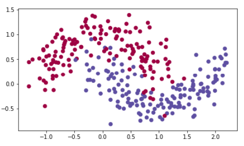
加载数据集
train_X, train_Y = load_dataset()
定义模型
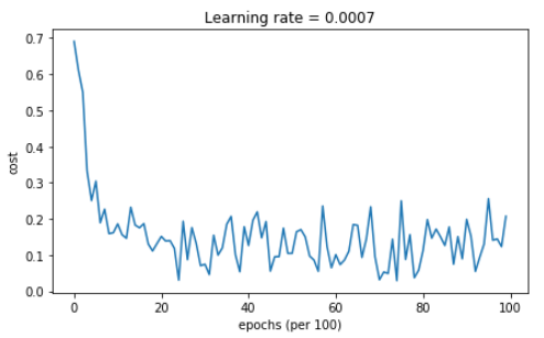
 1 def model(X, Y, layers_dims, optimizer, learning_rate=0.0007, mini_batch_size=64, beta=0.9,
 2           beta1=0.9, beta2=0.999, epsilon=1e-8, num_epochs=10000, print_cost=True):
 3     """
 4     3-layer neural network model which can be run in different optimizer modes.
 5
 6     Arguments:
 7     X -- input data, of shape (2, number of examples)
 8     Y -- true "label" vector (1 for blue dot / 0 for red dot), of shape (1, number of examples)
 9     layers_dims -- python list, containing the size of each layer
10     learning_rate -- the learning rate, scalar.
11     mini_batch_size -- the size of a mini batch
12     beta -- Momentum hyperparameter
13     beta1 -- Exponential decay hyperparameter for the past gradients estimates
14     beta2 -- Exponential decay hyperparameter for the past squared gradients estimates
15     epsilon -- hyperparameter preventing division by zero in Adam updates
16     num_epochs -- number of epochs
17     print_cost -- True to print the cost every 1000 epochs
18
19     Returns:
20     parameters -- python dictionary containing your updated parameters
21     """
22
23     L = len(layers_dims)             # number of layers in the neural networks
24     costs = []                       # to keep track of the cost
25     t = 0                            # initializing the counter required for Adam update
26     seed = 10                        # For grading purposes, so that your "random" minibatches are the same as ours
27
28     # Initialize parameters
29     parameters = initialize_parameters(layers_dims)
30
31     # Initialize the optimizer
32     if optimizer == "gd":
33         pass # no initialization required for gradient descent
34     elif optimizer == "momentum":
35         v = initialize_velocity(parameters)
36     elif optimizer == "adam":
37         v, s = initialize_adam(parameters)
38
39     # Optimization loop
40     for i in range(num_epochs):
41
42         # Define the random minibatches. We increment the seed to reshuffle differently the dataset after each epoch
43         seed = seed + 1
44         minibatches = random_mini_batches(X, Y, mini_batch_size, seed)
45
46         for minibatch in minibatches:
47
48             # Select a minibatch
49             (minibatch_X, minibatch_Y) = minibatch
50
51             # Forward propagation
52             a3, caches = forward_propagation(minibatch_X, parameters)
53
54             # Compute cost
55             cost = compute_cost(a3, minibatch_Y)
56
57             # Backward propagation
58             grads = backward_propagation(minibatch_X, minibatch_Y, caches)
59
60             # Update parameters
61             if optimizer == "gd":
62                 parameters = update_parameters_with_gd(parameters, grads, learning_rate)
63             elif optimizer == "momentum":
64                 parameters, v = update_parameters_with_momentum(parameters, grads, v, beta, learning_rate)
65             elif optimizer == "adam":
66                 t = t + 1 # Adam counter
67                 parameters, v, s = update_parameters_with_adam(parameters, grads, v, s,
68                                                                t, learning_rate, beta1, beta2,  epsilon)
69
70         # Print the cost every 1000 epoch
71         if print_cost and i % 1000 == 0:
72             print("Cost after epoch %i: %f" % (i, cost))
73         if print_cost and i % 100 == 0:
74             costs.append(cost)
75
76     # plot the cost
77     plt.plot(costs)
78     plt.ylabel('cost')
79     plt.xlabel('epochs (per 100)')
80     plt.title("Learning rate = " + str(learning_rate))
81     plt.show()
82
83     return parameters
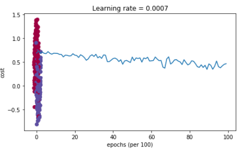
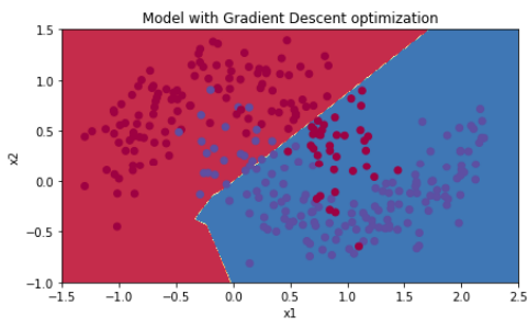
批量梯度下降
 1 # train 3-layer model
 2 layers_dims = [train_X.shape[0], 5, 2, 1]
 3 parameters = model(train_X, train_Y, layers_dims, optimizer="gd")
 4
 5 # Predict
 6 predictions = predict(train_X, train_Y, parameters)
 7
 8 # Plot decision boundary
 9 plt.title("Model with Gradient Descent optimization")
10 axes = plt.gca()
11 axes.set_xlim([-1.5, 2.5])
12 axes.set_ylim([-1, 1.5])
13 plot_decision_boundary(lambda x: predict_dec(parameters, x.T), train_X, train_Y)
预测准确度:0.797
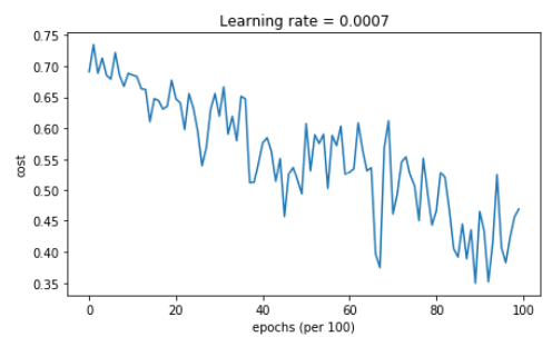
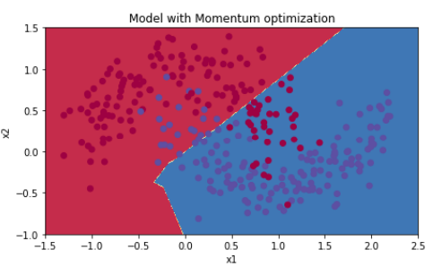
动量梯度下降
 1 # train 3-layer model
 2 layers_dims = [train_X.shape[0], 5, 2, 1]
 3 parameters = model(train_X, train_Y, layers_dims, beta=0.9, optimizer="momentum")
 4
 5 # Predict
 6 predictions = predict(train_X, train_Y, parameters)
 7
 8 # Plot decision boundary
 9 plt.title("Model with Momentum optimization")
10 axes = plt.gca()
11 axes.set_xlim([-1.5, 2.5])
12 axes.set_ylim([-1, 1.5])
13 plot_decision_boundary(lambda x: predict_dec(parameters, x.T), train_X, train_Y)
预测准确率:0.797
Adam梯度下降
 1 # train 3-layer model
 2 layers_dims = [train_X.shape[0], 5, 2, 1]
 3 parameters = model(train_X, train_Y, layers_dims, optimizer="adam")
 4
 5 # Predict
 6 predictions = predict(train_X, train_Y, parameters)
 7
 8 # Plot decision boundary
 9 plt.title("Model with Adam optimization")
10 axes = plt.gca()
11 axes.set_xlim([-1.5, 2.5])
12 axes.set_ylim([-1, 1.5])
13 plot_decision_boundary(lambda x: predict_dec(parameters, x.T), train_X, train_Y)
预测准确度:0.94