模型性能指标
作者:elfin 资料来源:mocro wen
1、前言--混淆矩阵
混淆矩阵主要预测-实际之间的混淆程度,并通过各种指标对这些结果的优劣程度进行度量。
1.1 二分类的混淆矩阵

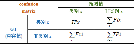
表1 二分类混淆矩阵
这里需要注意:
-
混淆矩阵的横坐标是预测值,纵坐标是真实值;
-
与笛卡尔坐标系相比,纵坐标保持01、横坐标是10;
-
在混淆矩阵中我们主要关注主对角线上的元素要尽可能大,
次对角线尽可能为0,即希望混淆矩阵是主对角矩阵;
-
混淆矩阵的元素TP、TN、FP、FN都是从左到右的读法,
第一个字母表示真假,第二个表示预测的情况;
具体含义见下面的列表。
混淆矩阵的符号含义:
- TP(True Positive):将正类预测为正类,即真实为1、预测也为1;
- FN(False Negative):将正例预测为负例,即真实为1,预测为0;
- FP(False Positive):将负例预测为正例,即真实为0,预测为1;
- TN(True Negative):将负例预测为负例,即真实为0,预测也为0.
Positive:积极的,这里表示阳性;
Negative:悲观的,这里表示阴性。
1.2 多分类的混淆矩阵
多分类的混淆矩阵:

这里的定义规则与二分类保持一致,两两之间或者x类别与非x类之间可以参考二分类绘制。
x类别与非x类之间的二分混淆矩阵:
1.3 python绘制混淆矩阵
使用python生成混淆矩阵
import random
from sklearn.metrics import confusion_matrix

labels = ["dog", "cat"]
y_true = [labels[round(random.random())] for _ in range(10)]
y_pred = [labels[round(random.random())] for _ in range(10)]
confusion_matrix1 = confusion_matrix(y_true=y_true,
                                     y_pred=y_pred,
                                     labels=labels)
print(f"y_true: {y_true}")
print(f"y_pred: {y_pred}")
print(confusion_matrix1)
输出:
y_true: ['cat', 'cat', 'cat', 'cat', 'cat', 'cat', 'dog', 'dog', 'dog', 'dog']
y_pred: ['dog', 'cat', 'dog', 'cat', 'cat', 'dog', 'dog', 'cat', 'cat', 'cat']
[[1 3]
 [3 3]]
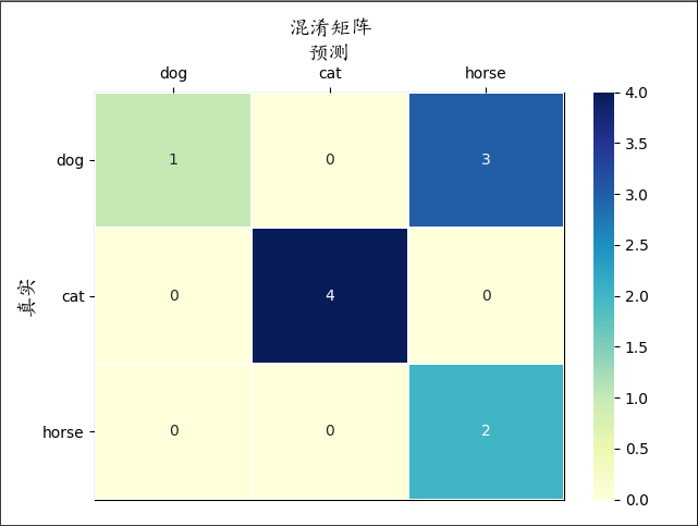
绘制混淆矩阵
这里自定义了一个class,封装了confusion_matrix与seaborn的热力图。效果图如下:
2、精确率Precision
精确率Precision:精确率又称查准率,指预测的正例结果中有多少是正确的!
(P=frac{TP}{TP+FP})
3、召回率Recall
召回率Recall:召回率又称查全率,指真实的正样本中有多少被正确查找到了!
(R=frac{TP}{TP+FN})
4、AP(Average precision) 平均精确度
在查阅资料时,遇到将AP、mAP混为一谈的,为了加以区分,我们从其本质介绍,不管是在哪个数据集(COCO)上的评测。
首先是Average precision,从字面理解我们会得到很多精确度,再对其求平均。此时有两种情况:
- Precision是某个指标的连续函数(非严格定义,可以理解为precision的值非离散),那么此时AP即为Precision的积分;
- Precision是某个指标的离散函数,即precision的值离散,此时AP即为“期望”(要注意实际上并不是求分布的期望).
为了方便理解,此处以BBox回归为例进行说明!
在目标检测任务中,往往需要对物体的bbox进行回归。这里我们需要使用Recall召回率、IOU值,前者在上面已经说明,而IOU值是目标检测中常用的指标。IOU值即为两个BBox的交与并的比值。在目标识别的场景中,我们可以分为以下两种情况:
- 只关注BBox是否正确锚定实例;
- 显著性水平是否达标,即得分score是否超过阈值.
本节我们只关注AP指标如何求,下面分别从二分类和MaskRCNN的角度讲解。
4.1 分类场景下的 AP
可参考资源AP和mAP的详解
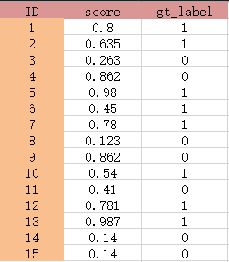
4.1.1 计算预测得分及其真实标签展示
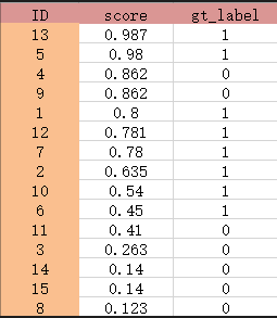
4.1.2 根据得分的高低按降序排列
4.1.3 Precision列表和Recall列表
Precisions = [1, 1 , 0.66666667, 0.5  , 0.6, 0.66666667 , 0.71428571,
              0.75 , 0.77777778 , 0.8 , 0.72727273, 0.66666666 ,
              0.61538461 , 0.57142857, 0.53333333]
Recalls = [0.06666667, 0.13333334, 0.13333334, 0.13333334, 0.2,
           0.26666668, 0.33333334, 0.4       , 0.46666667, 0.53333336,
           0.53333336, 0.53333336, 0.53333336, 0.53333336, 0.53333336]
4.1.4 计算AP
step1: 寻找召回率阶跃的点的索引indices
indices=[1, 4, 5, 6, 7, 8, 9]
step2_0:计算平均精度
若将Recalls看做横坐标、Precisions看做纵坐标,两者满足函数关系,则(AP)即可近似看为其期望!
step2_1:另一种常见的计算方法:
在每个召回率中取最大的精度求平均

上表中的绿色部分代表被我们选出来用于平均的值,所以:
AP=(1+1+0.66666667+0.5+0.6+0.66666667+0.71428571+0.75+0.77777778+0.8)/8=0.93442460375
4.2 Mask-RCNN的AP值
MaskRCNN在计算AP值时,使用的标记的mAP!
4.2.1 Mask-RCNN的AP值计算部分
	# Get matches and overlaps
    gt_match, pred_match, overlaps = compute_matches(
        gt_boxes, gt_class_ids, gt_masks,
        pred_boxes, pred_class_ids, pred_scores, pred_masks,
        iou_threshold)

    # Compute precision and recall at each prediction box step
    precisions = np.cumsum(pred_match > -1) / (np.arange(len(pred_match)) + 1)
    recalls = np.cumsum(pred_match > -1).astype(np.float32) / len(gt_match)

    # Pad with start and end values to simplify the math
    precisions = np.concatenate([[0], precisions, [0]])
    recalls = np.concatenate([[0], recalls, [1]])

    # Ensure precision values decrease but don't increase. This way, the
    # precision value at each recall threshold is the maximum it can be
    # for all following recall thresholds, as specified by the VOC paper.
    for i in range(len(precisions) - 2, -1, -1):
        precisions[i] = np.maximum(precisions[i], precisions[i + 1])

    # Compute mean AP over recall range
    indices = np.where(recalls[:-1] != recalls[1:])[0] + 1
    mAP = np.sum((recalls[indices] - recalls[indices - 1]) *
                 precisions[indices])
compute_matches函数先对预测的得分进行排序,根据得分从高到低对预测的pred_boxes、pred_class_ids、pred_masks进行一 一映射(重新排序);使用compute_overlaps_masks函数对mask矩阵进行两两间的IOU值,其参数为:masks1, masks2: [Height, Width, instances];所以再根据IOU值(overlaps:每个元素代表匹配到的实例集合),对每个overlaps元素进行排序(倒序:从大到小),再删除得分低于阈值的元素索引,在未删除的索引中进行预测和真实的匹配!
4.2.2 按得分从大到小排序
pred_boxes、pred_class_ids、pred_masks根据score排序后的索引更新,即他们依据score的顺序相应变化;
所以,此时Mask矩阵在通道维度上是有顺序的!
4.2.3 计算Pred_Masks与True_Masks之间的Iou值
预测的每一个mask与真实的每一个mask,两两计算Iou值,可以得到依据矩阵:
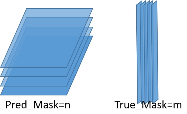
如图所示,n个预测的mask与m个真实的mask之间进行比较,会得到一个Iou值矩阵,将其命名为overlaps,shape=(n,m)。
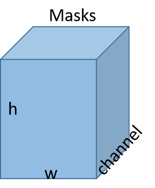
# 先将预测与真实的Mask数组平铺成 shape=(h*w, num_mask),注意平铺后的矩阵每一列就是一个Mask的所有元素,而masks1 > .5是用于生成True、False矩阵
masks1 = np.reshape(masks1 > .5, (-1, masks1.shape[-1])).astype(np.float32)
masks2 = np.reshape(masks2 > .5, (-1, masks2.shape[-1])).astype(np.float32)
area1 = np.sum(masks1, axis=0)
area2 = np.sum(masks2, axis=0)

# intersections and union
# 此时的masks1.T的shape为 (n, h*w); masks2的shape为(h*w, m)
intersections = np.dot(masks1.T, masks2)
union = area1[:, None] + area2[None, :] - intersections
overlaps = intersections / union
注意:每个实例的mask,背景为黑色,实例为白色,归一化后,实例部分应该是大于0.5的,所以求和后即为Mask区域的面积;相乘之后即为两个mask实例的并的面积!所以overlaps是一个Iou值矩阵,shape为(n,m)。
4.2.4 生成pred_match、gt_match
根据预测的bbox、真实的bbox的个数分别生成全为(-1)的pred_match、gt_match一维数组!
对预测维度n进行循环,每次取overlaps[i],即一个预测mask与所有真实的Mask之间的Iou值数组,将其值从大到小进行排序得到sorted_ixs,按Iou值排序后的顺序取值与阈值进行比较,得到不满足的sorted_ixs索引low_score_idx!
>>> a = np.array([[0.12, 0.53, 0.64, 0.31, 0.89, 0.45, 0.99, 0.06],[0.12, 0.53, 0.64, 0.31, 0.89, 0.45, 0.99, 0.06]])
>>> a
Out[19]:
array([[0.12, 0.53, 0.64, 0.31, 0.89, 0.45, 0.99, 0.06],
       [0.12, 0.53, 0.64, 0.31, 0.89, 0.45, 0.99, 0.06]])
>>> sorted_ixs = np.argsort(a[1])[::-1]
>>> sorted_ixs
Out[21]: array([6, 4, 2, 1, 5, 3, 0, 7], dtype=int64)
>>> low_score_idx = np.where(a[1, sorted_ixs] < 0.5)[0]
>>> low_score_idx
Out[23]: array([4, 5, 6, 7], dtype=int64)
# 将不满足阈值的sorted_ixs元素去除
>>> if low_score_idx.size > 0:
        sorted_ixs = sorted_ixs[:low_score_idx[0]]
>>> sorted_ixs
Out[25]: array([6, 4, 2, 1], dtype=int64)

# 3. Find the match
for j in sorted_ixs:
    # sorted_ixs的元素j标识的是真实的第j个mask,如果这个mask已经匹配了,那么不再进行匹配!
    if gt_match[j] > -1:
        continue
    # If we reach IoU smaller than the threshold, end the loop
    iou = overlaps[i, j]
    if iou < iou_threshold:
        break
    # 当pred_bbox[i]与gt_bbox[i]都未匹配,且IOU值大于阈值,恰好预测类别与真实类别一样,则匹配成功,匹配数加1。
    if pred_class_ids[i] == gt_class_ids[j]:
        match_count += 1
        gt_match[j] = i
        pred_match[i] = j
        break

基于上面的代码段和逻辑,我们可以树立出如下信息:
gt_match:元素是真实的bbox匹配的预测框索引(这里是大于-1的),若没有匹配到即为(-1).
pred_match: 元素是预测的bbox匹配到的真实框的索引(这里是大于-1的),若没有匹配到即为(-1).
4.2.5Precision 和 Recall
# 计算这一步中的所有预测框预测准确的累积概率,np.cumsum是求累积和;
# np.cumsum(pred_match > -1)是预测正确的累积频数.
precisions = np.cumsum(pred_match > -1) / (np.arange(len(pred_match)) + 1)
# 计算真实的框有多少个被正确地预测了的累积概率
recalls = np.cumsum(pred_match > -1).astype(np.float32) / len(gt_match)

# Pad with start and end values to simplify the math
precisions = np.concatenate([[0], precisions, [0]])
recalls = np.concatenate([[0], recalls, [1]])

# 确保数组是单调递减的,为什么只有精确度需要修正?注意召回率是没有np.arange的!
for i in range(len(precisions) - 2, -1, -1):
    precisions[i] = np.maximum(precisions[i], precisions[i + 1])
4.2.6 AP
# 计算召回率函数里发生阶跃的值的索引
indices = np.where(recalls[:-1] != recalls[1:])[0] + 1
# 根据召回率发生阶跃的索引获取 召回率的改变量*精度;注意这种求法和求积分的形式是类似的!
mAP = np.sum((recalls[indices] - recalls[indices - 1]) *
             precisions[indices])
5、mAP值
在第四章的基础上,如果在求解的计数过程中,预测和真实的对照是基于特定的某一类,求解出来的AP值即为当前类的平均精确度,将所有类别的AP求和再取平均就得到了mAP!