之前对线性回归和逻辑回归的理论部分做了较为详细的论述,下面通过一些例子再来巩固一下之前所学的内容。
需要说明的是,虽然我们在线性回归中都是直接通过公式推导求出w和b的精确值,但在实际运用中基本上都会采用梯度下降法作为首选,因为用代码表示公式会比较繁琐,而梯度下降法只需要不断对参数更新公式进行迭代即可,用代码表示非常简单,且迭代次数基本上不会对性能有太大的拖累,所以下面我们也将采用梯度下降的方法。
使用线性回归模拟数据分布
了解数据初始分布情况
现有一个数据集(提取码:yim9),描述了一系列点的分布情况。我们先将初始的分布情况绘制出来,便于对数据有个整体的了解:
import pandas as pd
import numpy as np
import matplotlib.pyplot as plt
from sklearn.linear_model import LinearRegression

data = np.loadtxt('./data/linear_regression_data.txt', delimiter=',')
print(data[:10])  # 查看部分样本数据
data.shape        # 查看样本规模

# 将数据集转换成 y = w*x 的向量形式
x = np.c_[np.ones(data.shape[0]), data[:, 0]]  # 使用np.c_转换为列向量
y = np.c_[data[:, 1]]  # 1是给b留的位置

# 展示样本分布情况
plt.scatter(x[:, 1], y, color='green', marker='x', linewidth=1)
plt.xlabel('X')
plt.ylabel('Y')
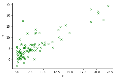
可以看到,点在X轴左侧分布得比较密集,但是越往右,越呈现出按照直线分布的趋势,所以可以尝试使用线性回归进行模拟。
使用最小二乘法构造目标函数
我们需要求出目标函数,以便求出梯度,并记录目标函数在每轮迭代中的值
# 目标函数
def target_func(x, y, w=[[0],[0]]):
    # 这里我们设置w和b的初始值为0
    h = x.dot(w)                                   # h表示预测值
    m = y.size                                     # 通常会使用样本大小m平均整体误差的值
    target = 1.0/(2*m) * (np.sum(np.square(h-y)))  # 使用最小二乘法得到目标函数
    return target
计算梯度及参数更新公式
# 计算梯度
def grad(x, y, w):
    h = x.dot(w)
    m = y.size
    grad = (1.0/m)*(x.T.dot(h-y))  # 对目标函数求导即是梯度
    return grad

# 使用梯度循环更新参数
def grad_descent(x, y, nums_iter=1000, n=0.01, w=[[0],[0]]):
    # 默认迭代1000次,学习率为0.01
    target_his = np.zeros(nums_iter)    # 存放目标函数每轮迭代后的值
    for i in np.arange(nums_iter):
        # 循环更新w,并记录目标函数的值
        w = w - n*grad(x, y, w)
        target_his[i] = target_func(x, y, w)
    return w, target_his

w, target_his = grad_descent(x, y)

# 展示迭代效果
plt.plot(target_his)
plt.xlabel('Iter Times')
plt.ylabel('Loss Function')
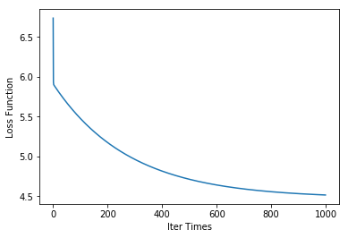
可以看出,迭代1000次,性能逐渐趋于平稳。
最后与sklearn的结果相对比:
# 样本
plt.scatter(x[:, 1], y, color='red', marker='x', linewidth=1)
# 自主
xx = np.arange(5, 23)
yy = w[0] + xx*w[1]
plt.plot(xx, yy, label='LD(GR)')

# sklearn
regr = LinearRegression()
# reshape转换成列向量
regr.fit(x[:, 1].reshape(-1, 1), y.ravel())
yy2 = regr.intercept_ + regr.coef_ * xx
plt.plot(xx, yy2, label='LD(sklearn)')

plt.xlim(4, 24)
plt.xlabel('X')
plt.ylabel('Y')
plt.legend(loc=4)
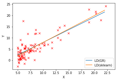
可以看出效果基本一致。
使用逻辑回归分类
现有一个考试成绩数据集(提取码:7n04),该数据集为某班级英语和数学两个科目的考试成绩,前两列分别表示英语和数学成绩,最后一列表示最终是否通过。
加载数据,查看数据样本及可视化
import pandas as pd
import numpy as np
import matplotlib as mpl
import matplotlib.pyplot as plt
from scipy.optimize import minimize

# Step 1. 加载数据
def loaddata(data):
     return np.loadtxt(data, delimiter=',')

data = loaddata('./data/sample_1.txt')
# 查看数据
print(data.shape)
print(data[:5, :])

# 运行结果:
(100, 3)
[[34.62365962 78.02469282  0.        ]
 [30.28671077 43.89499752  0.        ]
 [35.84740877 72.90219803  0.        ]
 [60.18259939 86.3085521   1.        ]
 [79.03273605 75.34437644  1.        ]]
# Step 2. 整理训练样本
# np.c_是按行连接两个矩阵,就是把两矩阵左右相加,要求行数相等
X = np.c_[np.ones((data.shape[0],1)), data[:,0:2]]
y = np.c_[data[:,2]]
print(X[:5])
print(X.shape)
print(y[:5])

# 运行结果:
[[ 1.         34.62365962 78.02469282]
 [ 1.         30.28671077 43.89499752]
 [ 1.         35.84740877 72.90219803]
 [ 1.         60.18259939 86.3085521 ]
 [ 1.         79.03273605 75.34437644]]
(100, 3)
[[0.]
 [0.]
 [0.]
 [1.]
 [1.]]
X的第一列是给偏置b预留的,其余两列为特征值。
# Step 3. 可视化
def plotData(data, label_x, label_y, label_pos, label_neg, axes=None):
    # 获得正负样本的下标(正样本表示考试通过的,负样本表示考试未通过)
    neg = data[:,2] == 0
    pos = data[:,2] == 1
    if axes == None:
        axes = plt.gca() # 获取图的坐标信息

    # 依次绘制正负样本,使用不同颜色区分
    axes.scatter(data[pos][:,0], data[pos][:,1], marker='*', c='r', s=30, linewidth=2, label=label_pos)
    axes.scatter(data[neg][:,0], data[neg][:,1], c='c', s=30, label=label_neg)
    axes.set_xlabel(label_x)
    axes.set_ylabel(label_y)
    axes.legend(frameon= True, fancybox = True);

plotData(data, 'English', 'Math', 'Pass', 'Fail')
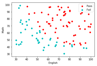
从样本分布可以看出,正负样本分布的还算整齐,可以使用决策边界进行划分。
定义Sigmoid函数、损失函数(即目标函数)、梯度函数
# Step 4. 训练前准备
# Sigmoid函数
def sigmoid(z):
    return(1 / (1 + np.exp(-z)))

# 损失函数
def lossFunction(w, X, y):
    m = y.size
    h = sigmoid(X.dot(w.reshape(-1, 1)))
    # 套公式得到损失函数
    J = -1.0*(1.0/m)*(np.log(h).T.dot(y)+np.log(1-h).T.dot(1-y))
    if np.isnan(J[0]):
        return(np.inf)
    return J[0]

# 梯度计算函数
def gradient(X, y, w):
    grad = np.zeros(w.shape)
    error = (sigmoid(X.dot(w.reshape(-1, 1))).reshape(-1, 1) - y).ravel()
    for j in range(len(w.ravel())):
        # 循环更新w,得到梯度
        term = np.multiply(error, X[:,j])
        grad[j] = np.sum(term) / len(X)
    return grad

# 初始化w
initial_w = np.zeros(X.shape[1])
loss = lossFunction(initial_w, X, y)
grad = gradient(X, y, initial_w)
print('Loss:
', loss)
print('Grad:
', grad)

# 输出结果:
Loss:
 [0.69314718]
Grad:
 [ -0.1        -12.00921659 -11.26284221]
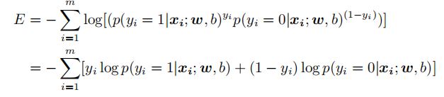
关于损失函数,代码里使用的是下面这个公式,而不是之前推导到最后的公式,因为用代码更好实现:
使用梯度下降法训练
# step 5. 使用梯度下降法训练
# 梯度下降函数
def gradientDescent(X, y, w, alpha=0.01, num_iters=1000):
    m = y.size
    J_history = np.zeros(num_iters)
    for iter in np.arange(num_iters):
        h = X.dot(w.reshape(-1, 1))
        grad = gradient(X, y, w)
        w = w - alpha*(1.0/m)*grad
        J_history[iter] = lossFunction(w, X, y)
    return(w, J_history)

# 画出每一次迭代和损失函数变化
w , Cost_J = gradientDescent(X, y, initial_w, alpha=0.15, num_iters=100000)

plt.plot(Cost_J)
plt.ylabel('Loss J')
plt.xlabel('Iter')
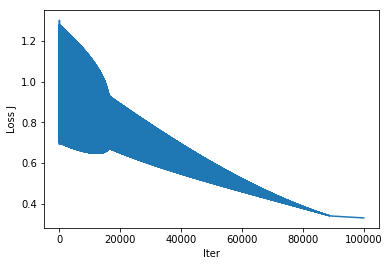
通过将学习率设置为0.15,并经过10W次的迭代后,损失函数计算出来的误差控制在了0.32左右。
下面对迭代出来的w进行可视化。
可视化决策边界
# Step 6. 可视化
plotData(data, 'English', 'Math', 'Pass', 'Fail')
# np.linspace(x1_min, x1_max) 生成的是x轴英语成绩的列向量
# np.linspace(x2_min, x2_max) 生成的是y轴数学成绩的列向量
# xx1, xx2为meshgrid生成的坐标矩阵
x1_min, x1_max = X[:,1].min(), X[:,1].max(),
x2_min, x2_max = X[:,2].min(), X[:,2].max(),
xx1, xx2 = np.meshgrid(np.linspace(x1_min, x1_max), np.linspace(x2_min, x2_max))
# 将预测值作为等高线绘制出来,即决策边界
# 将xx1和xx2作为x的特征值,得到预测值h
h = sigmoid(np.c_[np.ones((xx1.ravel().shape[0],1)), xx1.ravel(), xx2.ravel()].dot(w.T))
h = h.reshape(xx1.shape)
plt.contour(xx1, xx2, h, 1, linewidths=1, colors='b');
.png)
使用scipy.optimize.minimize实现
scipy.optimize.minimize可以根据现有的损失函数和梯度,优化整个梯度下降的过程,可以自动选择学习率,从而免去了不断手动调试的麻烦。
from scipy.optimize import minimize

res = minimize(lossFunction, initial_w, args=(X,y), jac=gradient, options={'maxiter':400})
print(res)
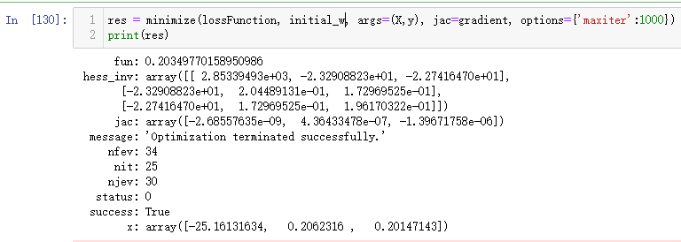
传入相应的参数,并设置迭代轮数(这里仅设置了400次),就可得到优化后的w。从输出可以看到,损失函数的误差已经减小到了0.2,比之前手动实现的要小很多,而且更加省时。
# Step 5. 可视化
plotData(data, 'English', 'Math', 'Pass', 'Fail')
x1_min, x1_max = X[:,1].min(), X[:,1].max(),
x2_min, x2_max = X[:,2].min(), X[:,2].max(),
xx1, xx2 = np.meshgrid(np.linspace(x1_min, x1_max), np.linspace(x2_min, x2_max))

h = sigmoid(np.c_[np.ones((xx1.ravel().shape[0],1)), xx1.ravel(), xx2.ravel()].dot(res.x.T))
h = h.reshape(xx1.shape)
plt.contour(xx1, xx2, h, 1, linewidths=1, colors='b');
.png)
从训练结果来看,手动和调包实现的效果好像差不多,但是明显后者更加省时省力。