参考:https://docs.rstudio.com/shinyapps.io/
1. 日期计算
链接:https://dingdangsunny.shinyapps.io/DateCalculate/
练习Shiny基本输入输出。
library(shiny)
ui <- fluidPage(
  titlePanel("使用Shiny进行日期计算"),
  h4(textOutput("currentTime")),
  helpText("请输入起止日期,计算日期间隔。"),
  helpText("默认计算当前日期与今年1月1日的间隔。"),
  dateRangeInput(inputId = "daterange", label = "日期范围:",
                 start = as.Date(paste(format(Sys.time()+8*60*60,
                                              "%Y"),
                                       "/01/01",sep = ""),
                                 "%Y/%m/%d"),
                 end = as.Date(format(Sys.time()+8*60*60,
                                      "%Y/%m/%d"),
                               "%Y/%m/%d")),
  textOutput("datedif"),
  tags$hr(),
  helpText("请输入起始日期和日期间隔,推算目标日期。"),
  helpText("(输入负数则为向前推算。)"),
  dateInput(inputId = "date", label = "起始日期:"),
  numericInput(inputId = "days", label = "日期间隔:",
               value = 100),
  textOutput("dateaft")
)
server <- function(input, output, session) {
  output$currentTime <- renderText({
    invalidateLater(1000, session)
    paste("当前时间是", Sys.time()+8*60*60)
  })
  output$datedif <- renderText({
    paste("相距", diff(input$daterange), "天")
  })
  output$dateaft <- renderText({
    d <- input$date + input$days
    paste("推算得日期为", d, format.Date(d,"%A"))
  })
}
shinyApp(ui = ui, server = server)
这里时间加8小时调整一下时区。
界面:
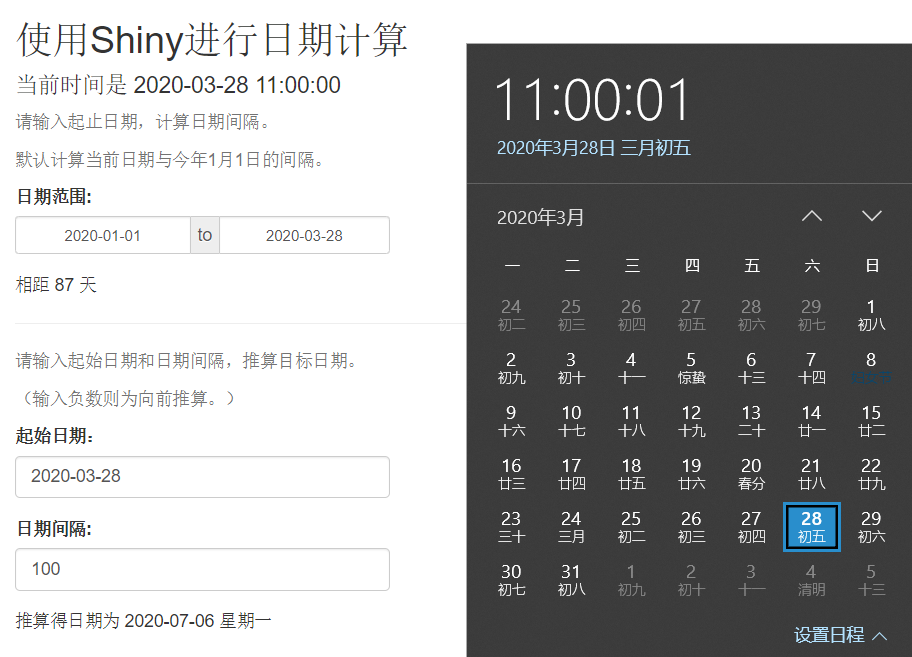
APP链接:https://dingdangsunny.shinyapps.io/DateCalculate/
2. FFT
关于FFT(快速傅里叶变换):https://www.cnblogs.com/dingdangsunny/p/12573744.html
链接:https://dingdangsunny.shinyapps.io/FastFourierTransform/
2.1 源代码
global.R
library(dplyr)
FFT<-function(data, Fs, isDetrend=TRUE)
{
  # 快速傅里叶变换
  # data:波形数据
  # Fs:采样率
  # isDetrend:逻辑值,是否进行去均值处理,默认为true
  # 返回[Fre:频率,Amp:幅值,Ph:相位(弧度)]
  n=length(data)
  if(n%%2==1)
  {
    n=n-1
    data=data[1:n]
  }
  if(n<4)
  {
    result<-data.frame(Fre=0,Amp=0,Ph=0)
    return(result)
  }
  if(isDetrend)
  {
    data<-scale(data,center=T,scale=F)
  }
  library(stats)
  Y = fft(data)
  #频率
  Fre=(0:(n-1))*Fs/n
  Fre=Fre[1:(n/2)]
  #幅值
  Amp=Mod(Y[1:(n/2)])
  Amp[c(1,n/2)]=Amp[c(1,n/2)]/n
  Amp[2:(n/2-1)]=Amp[2:(n/2-1)]/(n/2)
  #相位
  Ph=Arg(Y[1:(n/2)])
  result<-data.frame(Fre=Fre,Amp=Amp,Ph=Ph)
  return(result)
}
SUB<-function(t,REG)
{
  # 通过正则表达式提取输入数据
  m<-gregexpr(REG, t)
  start<-m[[1]]
  stop<-start+attr(m[[1]],"match.length")-1
  l<-length(start)
  r<-rep("1",l)
  for(i in 1:l)
  {
    r[i]<-substr(t,start[i],stop[i])
  }
  return(r)
}
#生成示例信号
deg2rad<-function(a)
{
  return(a*pi/180)
}
N = 256
Fs = 150
t = (0:(N-1))/Fs
wave = (5 + 8*cos(2*pi*10.*t) +
  4*cos(2*pi*20.*t + deg2rad(30)) +
  2*cos(2*pi*30.*t + deg2rad(60)) +
  1*cos(2*pi*40.*t + deg2rad(90)) +
  rnorm(length(t))) %>%
  paste(collapse = ",")
ui.R
library(shiny)
shinyUI(fluidPage(
titlePanel("使用Shiny进行FFT分析"),
sidebarLayout(
sidebarPanel(
selectInput(inputId = "input_mode",
label = "选择一种数据输入方式",
choices = c("文本输入", "上传文件")),
textAreaInput(inputId = "data",
label = "原始数据:",
value = wave,
rows = 10),
fileInput("file", "选择CSV文件进行上传",
multiple = FALSE,
accept = c("text/csv",
"text/comma-separated-values,text/plain",
".csv")),
checkboxInput("header", "是否有表头", TRUE),
radioButtons("sep", "分隔符",
choices = c("逗号" = ",",
"分号" = ";",
"制表符" = " "),
selected = ","),
numericInput(inputId = "Fs",
label = "采样频率:",
value = 150),
sliderInput("xlim", "x坐标范围:",
min = 0, max = 1,
value = c(0,1)),
sliderInput("ylim", "y坐标范围:",
min = 0, max = 1,
value = c(0,1)),
checkboxInput("isDetrend", "数据中心化", TRUE),
checkboxInput("showgrid", "添加网格线", TRUE)
),
mainPanel(
tabsetPanel(
type = "tabs",
tabPanel("图像", plotOutput(outputId = "data_in"),
plotOutput(outputId = "result")),
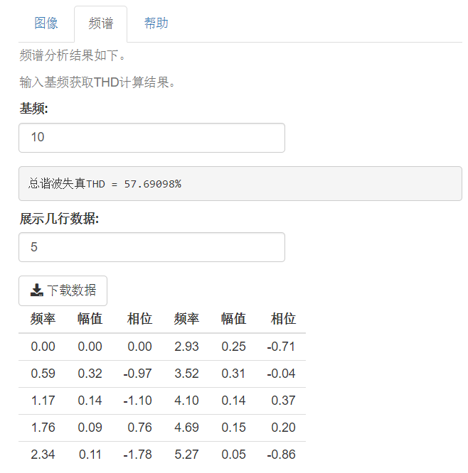
tabPanel("频谱",
helpText("频谱分析结果如下。"),
helpText("输入基频获取THD计算结果。"),
numericInput(inputId = "fund",
label = "基频:",
value = 10),
verbatimTextOutput("THD"),
numericInput(inputId = "num",
label = "展示几行数据:",
value = 15),
downloadButton("downloadData", "下载数据"),
tableOutput("resultview")
),
tabPanel("帮助",
helpText("这是一个基于Shiny创建的网页程序,
可以进行快速傅里叶变换(FFT)。",
"了解Shiny请访问:",
a(em("https://shiny.rstudio.com/"),
href="https://shiny.rstudio.com/")),
helpText("您可以选择在文本框中输入原始数据或通过CSV文件进行上传,
文本框中的数据应由逗号或空格分隔开,CSV中的数据应处于表格
的第一列。图像面板中向您展示了原始数据的序列和FFT变换后的结果,
通过x和y坐标范围的滑块,可以将分析结果的图形进行放大。
如果勾选了数据中心化的复选框,则将滤除直流成分,否则将保留。
在频谱面板中,可以查看FFT分析的数值结果并进行下载,通过输入基频,
可以获得总谐波失真(THD)计算结果。"),
helpText("源代码和演示示例请访问:",
a(em("叮叮当当sunny的博客"),
href="https://www.cnblogs.com/dingdangsunny/p/12586274.html#_label1"),
"")
)
)
)
)
))
server.R
library(shiny)
library(dplyr)
shinyServer(function(input, output) {
  data <- reactive({
    if(input$input_mode=="文本输入")
    {
      return(SUB(input$data,"[-0-9.]+") %>%
        as.numeric())
    }
    else if(input$input_mode=="上传文件")
    {
      req(input$file)
      data <- read.csv(input$file$datapath,
                        header = input$header,
                        sep = input$sep)
      return(data[,1])
    }
  })
  result <- reactive({
    FFT(data(), input$Fs, input$isDetrend)
  })
  output$data_in <- renderPlot({
    ylabel <- function()
    {
      if(input$input_mode=="上传文件" & input$header==TRUE)
        return((read.csv(input$file$datapath,
                        header = TRUE, sep = input$sep) %>%
                 names())[1])
      else
        return("value")
    }
    par(mai=c(1,1,0.5,0.5))
    plot((1:length(data()))/input$Fs, data(),
         type = "l", main = "The original data",
         xlab = "time/s", ylab = ylabel())
    if(input$showgrid)
    {
      grid(col = "darkblue", lwd = 0.5)
    }
  })
  output$result <- renderPlot({
    Fre_max <- max(result()$Fre)
    Amp_max <- max(result()$Amp)
    x_ran <- (input$xlim*1.1-0.05)*Fre_max
    y_ran <- (input$ylim*1.1-0.05)*Amp_max
    par(mai=c(1,1,0.5,0.5))
    plot(result()$Fre, result()$Amp, type = "l",
         xlab = "Frequency/Hz", ylab = "Amplitude",
         main = "FFT analysis results",
         xlim = x_ran, ylim = y_ran)
    if(input$showgrid)
    {
      grid(col = "darkblue", lwd = 0.5)
    }
  })
  output$resultview <- renderTable({
    r <- cbind(result()[1:input$num,],
               result()[(1+input$num):(2*input$num),])
    names(r) <- rep(c("频率", "幅值", "相位"), 2)
    r
  })
  output$THD <- renderPrint({
    n <- floor(dim(result())[1]/input$fund)
    A <- rep(0, n)
    for(i in 1:n)
    {
      A[i] <- result()$Amp[which(abs(result()$Fre-i*input$fund)==
                                   min(abs(result()$Fre-i*input$fund)))]
    }
    THD <- sqrt(sum((A[2:n])^2)/(A[1])^2)
    cat("总谐波失真THD = ",THD*100,"%",sep = "")
  })
  output$downloadData <- downloadHandler(
    filename = function() {
      return("FFTresult.csv")
    },
    content = function(file) {
      write.csv(result(), file)
    }
  )
})
2.2 测试
由默认数据集测试得到界面如下:

频率数据界面:
帮助文本界面:

用https://www.cnblogs.com/dingdangsunny/p/12573744.html#_label2中提到的数据进行文件上传测试。

APP链接:https://dingdangsunny.shinyapps.io/FastFourierTransform/
另外,发现了一个用Shiny写的有趣的小工具,http://qplot.cn/toolbox/,可以一试……