题目地址: http://openclassroom.stanford.edu/MainFolder/DocumentPage.php?course=DeepLearning&doc=exercises/ex2/ex2.html
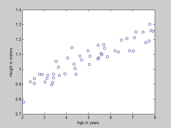
题目给出的数据是一组2-8岁男童的身高。x是年龄,y是身高。样本数m=50.
使用gradient descent来做线性回归。
step1:数据准备。
加载数据:
>> x=load('ex2x.dat');
>> y=load('ex2y.dat');
可视化数据:
figure % open a new figure window
plot(x, y, 'o');
ylabel('Height in meters')
xlabel('Age in years')
效果如下:
我们将模型设定为:
Hθ(x) = θ0 + θ1x
因此,还需要在数据集x的坐标统一加上1,相当于x0=1
m = length(y); % store the number of training examples
x = [ones(m, 1), x]; % Add a column of ones to x
增加了这一列以后,要特别注意,现在年龄这一变量已经移动到了第二列上。
step2:线性回归
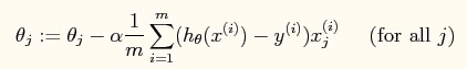
先来回忆一下我们的计算模型:
批量梯度下降(注意不是online梯度下降)的规则是:
题目要求:
1、使用步长为0.07的学习率来进行梯度下降。权重向量θ={θ0,θ1}初始化为0。计算一次迭代后的权重向量θ的值。
首先初始化权重向量theta
>> theta=zeros(1,2)
theta = 0 0
计算迭代一次时的权重向量:
delta=(x*theta')-y;
sum=delta'*x;
delta_theta=sum*0.07/m;
theta1=theta - delta_theta;
求得的theta1的结果为:
theta1 = 0.0745 0.3800
2、迭代进行gradient descent,直到收敛到一个点上。
测试代码(每100步输出一条theta直线,直到迭代结束):
function [ result ] = gradientDescent( x,y,alpha,accuracy )
%GRADIENTDESCENT Summary of this function goes here
%   Detailed explanation goes here
orgX=x;
plot(orgX, y, 'o');
ylabel('Height in meters')
xlabel('Age in years')
m=length(y);
x=[ones(m,1),x];
theta = zeros(1,2);
hold on;
times = 0;
while(1)
    times = times + 1;
    delta=(x*theta')-y;
    sum=delta'*x;
    delta_theta=sum*alpha/m;
    theta1=theta - delta_theta;
    if(all(abs(theta1(:) - theta(:)) < accuracy))
        result = theta;
        break;
    end
    theta = theta1;
    if(mod(times,100) == 0)
        plot(x(:,2), x*theta', '-','color',[(mod(times/100,256))/256 128/256 2/256]); % remember that x is now a matrix with 2 columns
        % and the second column contains the time info
        legend('Training data', 'Linear regression');
    end
end

end
效果如下:

可以看到,theta所确定的直线慢慢逼近数据集。
洁净版的代码(只输出最终的theta结果,不输出中间步骤):
function [ result ] = gradientDescent( x,y,alpha,accuracy )
%GRADIENTDESCENT Summary of this function goes here
%   Detailed explanation goes here
orgX=x;
plot(orgX, y, 'o');
ylabel('Height in meters')
xlabel('Age in years')
m=length(y);
x=[ones(m,1),x];
theta = zeros(1,2);
hold on;
while(1)
    delta=(x*theta')-y;
    sum=delta'*x;
    delta_theta=sum*alpha/m;
    theta1=theta - delta_theta;
    if(all(abs(theta1(:) - theta(:)) < accuracy))
        result = theta;
        plot(x(:,2), x*theta', '-','color',[200/256 128/256 2/256]); % remember that x is now a matrix with 2 columns
        % and the second column contains the time info
        legend('Training data', 'Linear regression');
        break;
    end
    theta = theta1;
end

end
结果:

执行代码
result=gradientDescent(x,y,0.07,0.00000001)
其中0.07为步长(即学习率),0.00000001为两个浮点矩阵的相近程度(即在这个程度内,视为这两个浮点矩阵相等)
收敛时的theta值为:
theta = 0.7502 0.0639
3、现在,我们已经训练出了权重向量theta的值,我们可以用它来预测一下别的数据。
predict the height for a two boys of age 3.5 and age 7
代码如下:
>> boys=[3.5;7];
>> boys=[ones(2,1),boys];
>> heights=boys*theta';
执行结果:
heights =
0.9737
1.1973
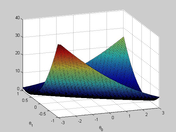
4、理解J(θ)
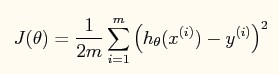
J(θ)是与权重向量相关的cost function。权重向量的选取,会影响cost的大小。我们希望cost可以尽量小,这样相当于寻找cost function的最小值。查找一个函数的最小值有一个简单的方法,就是对该函数求导(假设该函数可导),然后取导数为0时的点,该点即为函数的最小值(也可能是极小值)。梯度下降就是对J(θ)求偏导后,一步一步逼近导数为0的点的方法。
因为我们在此练习中使用的θ向量只有两个维度,因此可以使用matlab的plot函数进行可视化。在一般的应用中,θ向量的维度很高,会形成超平面,因此无法简单的用plot的方法进行可视化。
代码:
function [] = showJTheta( x,y )
%SHOW Summary of this function goes here
%   Detailed explanation goes here
J_vals = zeros(100, 100);   % initialize Jvals to 100x100 matrix of 0's
theta0_vals = linspace(-3, 3, 100);
theta1_vals = linspace(-1, 1, 100);
for i = 1:length(theta0_vals)
      for j = 1:length(theta1_vals)
      t = [theta0_vals(i); theta1_vals(j)];
      J_vals(i,j) = sum(sum((x*t - y).^2,2),1)/(2*length(y));
    end
end

% Plot the surface plot
% Because of the way meshgrids work in the surf command, we need to
% transpose J_vals before calling surf, or else the axes will be flipped
J_vals = J_vals'
figure;
surf(theta0_vals, theta1_vals, J_vals);
axis([-3, 3, -1, 1,0,40]);
xlabel('\theta_0'); ylabel('\theta_1')

end
执行:
x=load('ex2x.dat');
y=load('ex2y.dat');
x=[ones(length(y),1),x];
showJTheta(x,y);
结果
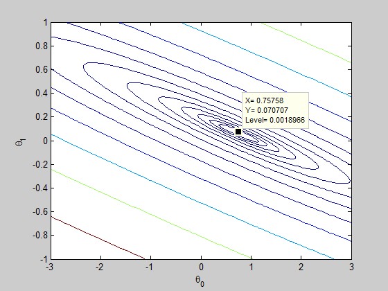
加上等高线的绘制语句
figure;
% Plot the cost function with 15 contours spaced logarithmically
% between 0.01 and 100
contour(theta0_vals, theta1_vals, J_vals, logspace(-2, 2, 15));
xlabel('\theta_0'); ylabel('\theta_1');
效果