Gao, S., Wu, J., Stiller, J. et al. Identifying barley pan-genome sequence anchors using genetic mapping and machine learning. Theor Appl Genet 133, 2535–2544 (2020). https://doi.org/10.1007/s00122-020-03615-y
作者采用了GBS测序方法,测定了11,166个栽培种和1140野生种大麦,通过读取64bp长度,分别获得了1800万和980万个原始GBS标签。对于这些标签,作者计算了tag的两个位置:①LD分析,取最相关的SNP作为其位置;②BWA比对,得到物理位置。通过比较这两个位置的距离差,将tag分为4类,其中第四类指距离差大于10Mbp的。由于该距离差过大,作者扔掉了第四类tag。通过机器学习,作者识别了信息不足的tag的分组信息,进而在大麦基因组Morex上识别了PAV tag。最后,作者使用这些标签对开花时间,植物高度和籽粒大小进行了GWAS分析,并得出结论:PAV和非PAV标签的相对重要性因不同性状而异;基于GBS标签的全基因组序列锚可以促进全面的全基因组的构建,并极大地协助各种遗传研究,包括结构变异的鉴定,遗传图谱和大麦的育种;PAV和非PAV标签的相对重要性因不同性状而异。
(本文的作者似乎采用“genotypes”代表样本?)

1. 方法
1.1 数据源
作者用到的数据包括:①作者自己测的GBS tag(Phred quality threshold of 30 and read length threshold of 64 bp)②下载的SNP矩阵和表型数据(https://doi.org/10.5447/IPK/2018/9,原文即区分了野生和栽培)
作者使用KMC(v3.0.0)从修剪后的读段中提取了k-mer大小为64bp且出现次数不少于30的作为GBS标签(补充图1a)。在所有genotypes中都出现的GBS tag被记录为一个“Unique Record”(UR),每个UR代表存在于同一基因型子集中的所有GBS标签。

Supplementary Figure 1 The pipeline used in generating the GBS tags and unique record (URs) used in linkage disequilibrium mapping. (a) K-mer analysis for each of the genotypes, and (b) Sorting GBS tags into URs.
1.2 基于LD对UR映射到SNP矩阵上(LDM)
作者首先使用了Tassel v5.0将下载的SNP矩阵从VCF转换为Hapmap格式,随后对每个UR,针对整个SNP矩阵计算并降序排列“ SUM”值。“ SUM”被设计为Cohen’s kappa statistics,以评估所有大麦基因型中SNP基因型与UR是否存在的一致性。
关联的SNP定义为:从最高的SUM值开始,并在所有七个染色体上的SNP以及unknown reads的集合出现在降序的排序结果中时停止。具有最高SUM值的关联SNP的位置被视为UR的LDM位置。

Supplementary Figure 2 Linkage disequilibrium mapping of unique records (URs) against the SNP matrix. The genotype list includes all genotypes used in the analysis. Unique Record i contains a subset of the genotypes. It is transformed into an ‘0-1’ binary sequence based on the genotype list, where ‘0’ stands for the presence of an UR in the genotype and ‘1’ stand for absence. The equation shows how ‘SUM’ is calculated between UR and a single SNP, where ‘M1’ represents the number of matched pairs of ‘1’ and a certain type of nucleotide and ‘M0’ means the number of matched pairs of ‘0’ and the other type of nucleotide. As each SNP locus contains binary nucleotide, there will be two ways to match ‘0’ and ‘1’ to nucleotides. Taking the SNP 1 as example, the match will be either ‘1-G and 0-T’ or ‘1-T and 0-G’. In the script ‘calculate_bino.pl’, we defined that the larger value generated by the two ways will be kept for each UR. Therefore, the closer the ‘SUM’ is to 2, the more consistent between the UR and a certain SNP is.
1.3 GBS tag的分组
UAMT的定义:使用BWA (version 0.7.15) mem 将所有GBS标签与Morex基因组进行比对,并将唯一且完全比对的标签定义为UAMT。最佳匹配的坐标是在相应GBS标签的物理位置获取的。
参照玉米中的模型训练结果,根据物理位置和LDM位置之间的距离(距离)将UAMT分为四类:第一类:Dist≤1000 bp;第二类:Dist≤1000 bp;2类:1000 bp <Dist≤100 Kbp; 3级:100 Kbp <Dist≤10 Mbp; 等级4:Dist≥10 Mbp。这种分组方法允许训练有素的RF分类器以不同的准确性水平预测GBS标签。
In the study reported here, we focused on results of Classes 1–3, which were defined as reliable tags.
1.4 机器学习模型的选择
作者评估研究了三种机器学习方法,即人工神经网络(ANN),支持向量分类器(SVC)和随机森林(RF)。通过比较,RF模型表现出最好的性能,因此,在本研究中,最终选择了RF模型对GBS标签进行分类。Python中的scikit-learn模块和Jupyter notebook一起用于训练RF模型。

Supplementary Figure 3 The machine learning algorithm comparison on the position confidence evaluation (wild dataset). As illustrated in above, the R (c and f) is superior to the ANNs (a and d) and SVC (b and e). For the ROC curve comparison, the AUC values for all four classes using the RF are significantly larger than these using the ANNs and the SVC. On the other hand, from the precision-recall curves, the difference among the RF, the ANNs, and SVC, are more remarkable, showing the RF is more efficient in the unbalanced data with high AUC values (Class 1: 0.93, Class 2: 0.80, Class 3: 0.71, and Class 4: 1.00). From above analysis, compared with the ANNs and the SVC, the RF is a more reliable machine learning method for the position confidence evaluation of the GWAS results.
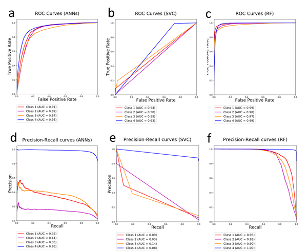
Supplementary Figure 4 The machine learning algorithm comparison on the position confidence evaluation (domesticated dataset). Like the results presented in the wild dataset, the RF model (c and f) showed better performance of classification than the ANNs (a and d) and the SVC models (b and e) in the domesticated dataset as well.
(然而,作者的ANN模型构建的极为简单,仅由三层构成,即输入层、隐藏层和输出层,而隐藏层仅有30个节点)
1.5 机器学习模型的训练
根据以下公式对所有位置进行转化:transformed position = chromosome × 1E9 + position。(相当于将不同染色体连起来,中间以若干N隔开)。
机器学习分类的准确性是通过RF模型在训练集上的out-of-bag cross-validation 评估的。作者随机选取了200,000个UAMT作为训练集,其中25%用来测试。该训练集用于生成ROC曲线和PRC曲线。最终使用的模型是基于全部UAMT训练的。
对每个UR,基于LDM result,计算了共10个feature。
| Feature | Description | Selection reason |
|---|---|---|
| Best_value | The best SUM value | Significance levels of association between tags and SNPs. |
| RatioM_odd | Odd ratio of SUM(best chromosome) vs SUM(median chromosome) | Spurious association due to population structures. True associations should have higher values of RatioM_odd. |
| Ratio2ed_odd | Odd ratio of SUM(best chromosome) vs SUM(second-best chromosome) | Levels of spurious associations due to population structures. True association should have higher values of Ratio2ed_odd. |
| G_width | Physical distance between the first and last significant SNPs on the best chromosome | Sizes of LD blocks. |
| Total_Sig_Num | Total number of significant SNPs | SNPs associated with population structures and repetitiveness of tags. |
| Sig_Num_BestChr | Total number of significant SNPs on the best chromosome | SNPs associated with population structures and levels of confidence in association tests. |
| Sig_Num_BC_percent | Sig_Num_BC / Total_Sig_Num | Associated with population structure and confidence levels in association tests. True association should have higher Sig_Num_BC_percent. |
| RatioGSN | G_width / Sig_Num_BC | Sizes of LD blocks, population structures and confidence levels in association tests. |
| RootGSN | G_width ^ (1 / Sig_Num_BC ) | Associated with sizes of LD blocks, population structures and confidence levels of association tests. |
| TaxaCount | Number of genotypes in which the tag is detected | Associated with the repetitiveness and frequency of the tags. |
RF训练参数为n_estimators = 90; min_samples_leaf = 2; max_features = 6,其他保留默认参数。
RF模型被用于推测分组未知的GBS tag。
1.6 PAV标签
在标记为1-3类的标签中,Morex参考基因组中不存在的标签被定义为PAV-I标签。LDM位置与其物理位置的每次命中均相距100 Mb的标签被定义为PAV-II标签。
为了验证PAV-I标签的可信度,作者使用BWA mem将其与the hulless barley genotype(Zangqing320)的基因组比对,并滤出了具有完美比对的基因(ZQ标签)。然后,作者将ZQ标签周围的Zangqing320的2 Kb侧翼序列比对回到了Morex基因组。如果侧翼序列在给定ZQ标签的LDM位置的10 Mbp范围内比对,则视为成功验证(补充图5)。

Supplementary Figure 5 Validation strategy for PAV-I tags. The red stars indicated the LDM positions of the PAV-I tags.
1.7 GWAS
using GAPIT v2.0
GWAS分析中,将与GBS tag关联最紧密的SNP当作该tag,进行关联研究。
2. 随机森林的分类结果
经过所有UAMT训练的最终RF模型应用于驯化群体和野生群体GBS标签的所有LDM结果。总共1,380,465个驯化和443,871个野生GBS标签被分为三个不同的类别(1、2和3),从此被视为pan-genome sequence anchors。其中,来自栽培数据集的66.8%和来自野生数据集的83.4%是Non-PAV标签(图 3a,c),因为它们在Morex基因组上的物理位置与LDM位置相同(图 3 b,d)。这些结果提供了进一步的证据,表明了RF分类器的稳健性和可信性。
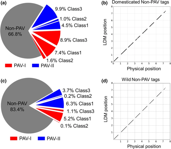
Fig. 3 Classification results of random forest classifiers. The pie charts show the proportions of three types of tags from a domesticated dataset and c wild dataset. The scatter plots show the physical positions against linkage disequilibrium mapping (LDM) positions of the non-PAV tags from b the domesticated and d wild datasets. The numbers on x- and y-axis indicate barley chromosomes (‘8’ indicates the unknown chromosome). All positions are transformed using the equation: transformed position = chromosome × 1E9 + position
3. PAV标签的全基因组分布
来自栽培和野生数据集的PAV-I标签共享相似的染色体范围分布模式(图 4a,c)。这些标签中的大多数位于染色体的远端区域,而在着丝粒附近区域仅发现了少数。PAV-II标签的分布与PAV-I相似,但前者在大部分染色体的远侧区的密度甚至更高(图的 4 B,d)(野生和栽培均显示此特征)。有趣的是,少数栽培数据集中的PAV-II标签均位于染色体1H的近着丝粒的区域(图 4 b)中,这与野生群体不一致。
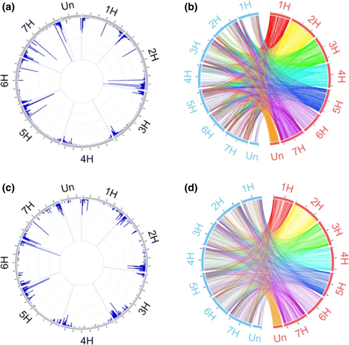
Fig. 4 Genome-wide distribution of PAV tags. a Domesticated PAV-I tags. The highest bar represents 10,000 tags; b domesticated PAV-II tags. The physical and LDM positions are shown in red and cyan, respectively; c wild PAV-I tags. The highest bar represents 1200 tags; d wild PAV-II tags. The physical and LDM positions are shown in red and cyan, respectively (color figure online)
4. GWAS分析结果
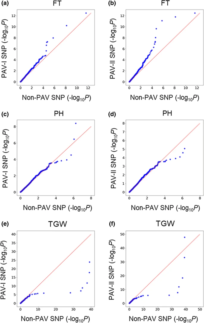
Q–Q plot of pairwise comparison of GWAS hits between non-PAV SNPs and PAV SNPs. a, c, e non-PAV SNPs versus PAV-I SNPs. b, d, f non-PAV SNPs versus PAV-II SNPs. ‘FT’ stands for flowering time; ‘PH’ stands for plant height; ‘TGW’ stands for thousand grain weight
5. 结果
在这项研究中,作者确定了180万个大麦泛基因组序列锚点,覆盖了11166株驯化的大麦和1140株野生大麦。总共确定了532,253个PAV变异标签,它们提供了大麦中全基因组PAV分布的概述。作者的发现表明,PAV可以显着影响大麦开花时间。这些PAV标签将有助于各种遗传学研究,包括鉴定大麦的结构变异,遗传作图和标记发育。此外,这些泛基因组序列锚点可以通过定位无法单独计算放置的支架/转录本,来帮助构建全面的大麦泛基因组。