这里有一篇原作者的博客:深入浅出Tensorflow(四):卷积神经网络
6.2 卷积神经网络简介
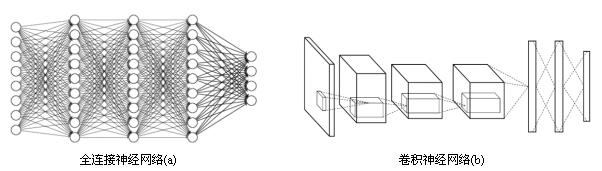
卷积神经网络和全连接神经网络的整体架构非常相似,唯一区别就在于神经网络中相邻两层的连接方式,相邻两层之间只有部分节点相连,为了展示每一层神经元的维度,一般将每一层卷积层的节点组织成一个三维矩阵。
使用全连接神经网络处理图像的最大问题在于全连接层的参数太多,对于MNIST数据,一个全连接层的神经网络有28*28*500+500=392500个。如果考虑Cifar-10数据集,图片大小为32*32*3,这样输入层有3072个节点,如果全连接层仍有500个节点,那么这一层全连接神经网络将有3072*500+500≈150w个参数,参数增多既会导致计算速度减慢还很容易导致过拟合问题。
一个卷积神经网络主要由以下五种结构组成:
- 输入层:一般代表一张图片的像素矩阵。其中三维矩阵的长和宽代表了图像的大小,深度代表了图像的彩色通道。
- 卷积层:卷积层每一个节点的输入只是上一层神经网络的一小块,常用3*3、5*5,可以得到抽象程度更高的特征。一般来说,通过卷积层处理的节点矩阵会变深。
- 池化层:不会改变三维矩阵的深度,但可以缩小矩阵的大小,可以认为是将图片的分辨率降低,通过池化层可以进一步缩小节点个数,减少整个神经网络的参数。
- 全连接层:在经过多轮卷积层和池化层处理之后(看作自动图像特征提取的过程),一般由1到2个全连接层来给出最后的分类结果。
- Softmax层:可以得到样例属于不同种类的概率分布情况。
6.3 卷积神经网络常用结构
(1)卷积层
过滤器(filter)可以将当前层神经网络的一个子节点矩阵转化为下一层神经网络上的一个单位节点矩阵(长和宽都为1,但深度不限)。
过滤器的尺寸指的是一个过滤器输入节点矩阵的大小,而深度指的是输出单位节点矩阵的深度。
想要调整结果矩阵的大小可以通过 全0填充 或 设置过滤器移动的步长。
在卷积神经网络中,每一个卷积层中使用的过滤器中的参数都是一样的,这是卷积神经网络一个非常重要的性质。
以Cifar-10为例,输入层维度32*32*3,卷积层使用尺寸5*5,深度为16,那么卷积层到的参数个数为5*5*3*16=1216个,而500个隐藏节点的全连接层将有150w个参数。
卷积层的参数个数和图片的大小无关,它只和过滤器的尺寸、深度以及当前节点矩阵的深度有关。
#卷积层的权重参数是一个4维矩阵,前两个维度代表过滤器的尺寸,第三个维度表示当前层的深度,第四个维度表示过滤器的深度。
filter_weight=tf.get_variable('weights',[5,5,3,16],initializer=tf.truncated_normal_initializer(stddev=0.1))
biases=tf.get_variable('biases',[16],initializer=tf.constant_initializer(0.1))
#f.nn.conv2d提供了实现卷积层向前传播的算法,第一个输入为当前层的节点矩阵,第一维对应输入batch,后三维对应一个节点矩阵,如input[0,:,:,:]
#表示第一张图片,第二个参数提供了卷积层的权重,第三个参数为不同维度上的步长,四维数组第一维和最后一维都是1,因为步长只对长和宽有效,
#最后一个参数是填充,SAME表示添加全0填充,VALID表示不添加
conv=tf.nn.conv2d(input,filter_weight,strides=[1,1,1,1],padding='SAME')
#矩阵上不同位置的节点都需要加上同样的偏执项,所以不能直接使用加法
bias=tf.nn.bias_add(conv,biases)
actived_conv=tf.nn.relu(bias)
(2)池化层
池化层可以非常有效地缩小矩阵的尺寸,从而减少最后全连接层中的参数。使用池化层可以加快计算速度也有防止过拟合问题的作用,一般池化层的过滤器采用最大值(常用)或平均值运算。
卷积层使用的过滤器是横跨整个深度的,而池化层使用的过滤器只影响一个深度上的节点,所以池化层的过滤器除了在长和宽两个维度移动之外,它还需要在深度这个维度移动。
#第一个参数为节点矩阵和tf.nn.conv2d函数的第一个参数一致,第二个参数为过滤器尺寸,最多的为[1,2,2,1],[1,3,3,1],第三个参数为步长,第四个参数指定是否使用全0填充
pool=tf.nn.max_pool(actived_conv,ksize=[1,3,3,1],strides=[1,2,2,1],padding='SAME')
(3)卷积层、池化层样例


import tensorflow as tf
import numpy as np

M = np.array([
        [[1],[-1],[0]],
        [[-1],[2],[1]],
        [[0],[2],[-2]]
    ])

print "Matrix shape is: ",M.shape
#Matrix shape is:  (3, 3, 1)
filter_weight = tf.get_variable('weights', [2, 2, 1, 1], initializer = tf.constant_initializer([
                                                                        [1, -1],
                                                                        [0, 2]]))
biases = tf.get_variable('biases', [1], initializer = tf.constant_initializer(1))
M = np.asarray(M, dtype='float32')
M = M.reshape(1, 3, 3, 1)
x = tf.placeholder('float32', [1, None, None, 1])
conv = tf.nn.conv2d(x, filter_weight, strides = [1, 2, 2, 1], padding = 'SAME')
bias = tf.nn.bias_add(conv, biases)
pool = tf.nn.avg_pool(x, ksize=[1, 2, 2, 1], strides=[1, 2, 2, 1], padding='SAME')
with tf.Session() as sess:
    tf.global_variables_initializer().run()
    convoluted_M = sess.run(bias,feed_dict={x:M})
    pooled_M = sess.run(pool,feed_dict={x:M})

    print "convoluted_M:
", convoluted_M
    print "pooled_M:
", pooled_M
-------------------------------------------------------------------------
convoluted_M:
[[[[ 7.]
   [ 1.]]

  [[-1.]
   [-1.]]]]
pooled_M:
[[[[ 0.25]
   [ 0.5 ]]

  [[ 1.  ]
   [-2.  ]]]]
这里我一开始对结果有较大疑问,因为与我用左上角全零填充算出来的结果不一致,通过对程序运行结果的逆推导,可以得到以下两个填充后的模型:
卷积层:
1, -1, 0, 0
-1, 2, 1, 0
0, 2, -2, 0
0, 0, 0, 0
池化层:
1, -1, 0, 0
-1, 2, 1, 1
0, 2, -2, -2
0, 2, -2, -2
6.4 经典卷积网络模型
(1)LeNet-5 模型
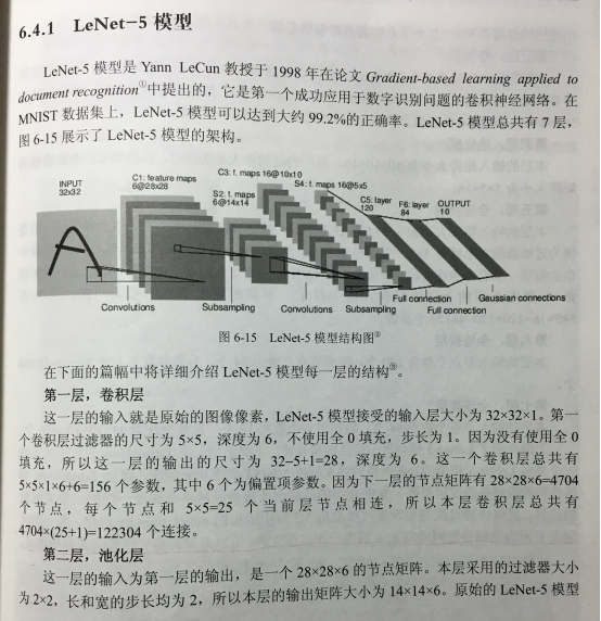
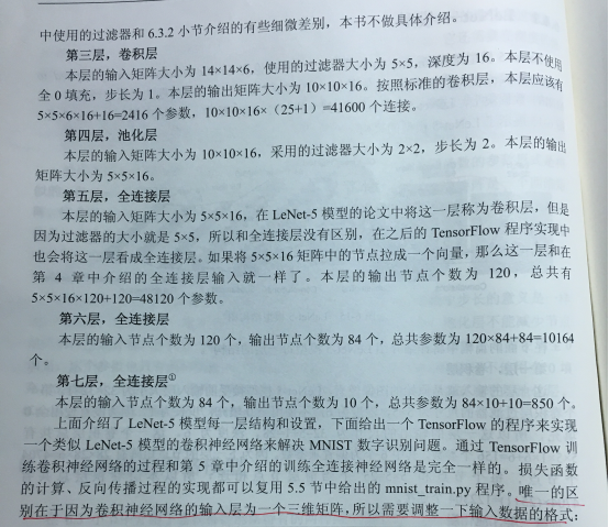
下面给出一个TensorFlow的程序来实现类似LeNet-5模型的卷积神经网络来解决MNIST数字识别问题。
这个程序中将用到dropout方法,dropout可以进一步提升模型可靠性并防止过拟合:TensorFlow学习---tf.nn.dropout防止过拟合
首先是修改的mnist_inference:
import tensorflow as tf
#1. 设定神经网络的参数
INPUT_NODE = 784
OUTPUT_NODE = 10

IMAGE_SIZE = 28
NUM_CHANNELS = 1
NUM_LABELS = 10

CONV1_DEEP = 32
CONV1_SIZE = 5

CONV2_DEEP = 64
CONV2_SIZE = 5

FC_SIZE = 512
#2. 定义前向传播的过程
def inference(input_tensor, train, regularizer):
    with tf.variable_scope('layer1-conv1'):
        conv1_weights = tf.get_variable(
            "weight", [CONV1_SIZE, CONV1_SIZE, NUM_CHANNELS, CONV1_DEEP],
            initializer=tf.truncated_normal_initializer(stddev=0.1))
        conv1_biases = tf.get_variable("bias", [CONV1_DEEP], initializer=tf.constant_initializer(0.0))
        conv1 = tf.nn.conv2d(input_tensor, conv1_weights, strides=[1, 1, 1, 1], padding='SAME')
        relu1 = tf.nn.relu(tf.nn.bias_add(conv1, conv1_biases))

    with tf.name_scope("layer2-pool1"):
        pool1 = tf.nn.max_pool(relu1, ksize = [1,2,2,1],strides=[1,2,2,1],padding="SAME")

    with tf.variable_scope("layer3-conv2"):
        conv2_weights = tf.get_variable(
            "weight", [CONV2_SIZE, CONV2_SIZE, CONV1_DEEP, CONV2_DEEP],
            initializer=tf.truncated_normal_initializer(stddev=0.1))
        conv2_biases = tf.get_variable("bias", [CONV2_DEEP], initializer=tf.constant_initializer(0.0))
        conv2 = tf.nn.conv2d(pool1, conv2_weights, strides=[1, 1, 1, 1], padding='SAME')
        relu2 = tf.nn.relu(tf.nn.bias_add(conv2, conv2_biases))

    with tf.name_scope("layer4-pool2"):
        pool2 = tf.nn.max_pool(relu2, ksize=[1, 2, 2, 1], strides=[1, 2, 2, 1], padding='SAME')
        pool_shape = pool2.get_shape().as_list()
        nodes = pool_shape[1] * pool_shape[2] * pool_shape[3]
        reshaped = tf.reshape(pool2, [pool_shape[0], nodes])

    with tf.variable_scope('layer5-fc1'):
        fc1_weights = tf.get_variable("weight", [nodes, FC_SIZE],
                                      initializer=tf.truncated_normal_initializer(stddev=0.1))
        if regularizer != None: tf.add_to_collection('losses', regularizer(fc1_weights))
        fc1_biases = tf.get_variable("bias", [FC_SIZE], initializer=tf.constant_initializer(0.1))

        fc1 = tf.nn.relu(tf.matmul(reshaped, fc1_weights) + fc1_biases)
        if train: fc1 = tf.nn.dropout(fc1, 0.5)

    with tf.variable_scope('layer6-fc2'):
        fc2_weights = tf.get_variable("weight", [FC_SIZE, NUM_LABELS],
                                      initializer=tf.truncated_normal_initializer(stddev=0.1))
        if regularizer != None: tf.add_to_collection('losses', regularizer(fc2_weights))
        fc2_biases = tf.get_variable("bias", [NUM_LABELS], initializer=tf.constant_initializer(0.1))
        logit = tf.matmul(fc1, fc2_weights) + fc2_biases

    return logit
损失函数的计算、反向传播过程的实现都可以复用5.5节中给出的mnist_train.py程序,为一个区别在于卷积神经网络的输入层为一个三维矩阵,所以需要调整以下输入数据的格式:
import tensorflow as tf
from tensorflow.examples.tutorials.mnist import input_data
import LeNet5_infernece
import os
import numpy as np
#1. 定义神经网络相关的参数
BATCH_SIZE = 100
LEARNING_RATE_BASE = 0.01
LEARNING_RATE_DECAY = 0.99
REGULARIZATION_RATE = 0.0001
TRAINING_STEPS = 6000
MOVING_AVERAGE_DECAY = 0.99
#2. 定义训练过程
def train(mnist):
    # 定义输出为4维矩阵的placeholder
    x = tf.placeholder(tf.float32, [
            BATCH_SIZE,
            LeNet5_infernece.IMAGE_SIZE,
            LeNet5_infernece.IMAGE_SIZE,
            LeNet5_infernece.NUM_CHANNELS],
        name='x-input')
    y_ = tf.placeholder(tf.float32, [None, LeNet5_infernece.OUTPUT_NODE], name='y-input')

    regularizer = tf.contrib.layers.l2_regularizer(REGULARIZATION_RATE)
    y = LeNet5_infernece.inference(x,False,regularizer)
    global_step = tf.Variable(0, trainable=False)

    # 定义损失函数、学习率、滑动平均操作以及训练过程。
    variable_averages = tf.train.ExponentialMovingAverage(MOVING_AVERAGE_DECAY, global_step)
    variables_averages_op = variable_averages.apply(tf.trainable_variables())
    cross_entropy = tf.nn.sparse_softmax_cross_entropy_with_logits(logits=y, labels=tf.argmax(y_, 1))
    cross_entropy_mean = tf.reduce_mean(cross_entropy)
    loss = cross_entropy_mean + tf.add_n(tf.get_collection('losses'))
    learning_rate = tf.train.exponential_decay(
        LEARNING_RATE_BASE,
        global_step,
        mnist.train.num_examples / BATCH_SIZE, LEARNING_RATE_DECAY,
        staircase=True)

    train_step = tf.train.GradientDescentOptimizer(learning_rate).minimize(loss, global_step=global_step)
    with tf.control_dependencies([train_step, variables_averages_op]):
        train_op = tf.no_op(name='train')

    # 初始化TensorFlow持久化类。
    saver = tf.train.Saver()
    with tf.Session() as sess:
        tf.global_variables_initializer().run()
        for i in range(TRAINING_STEPS):
            xs, ys = mnist.train.next_batch(BATCH_SIZE)

            reshaped_xs = np.reshape(xs, (
                BATCH_SIZE,
                LeNet5_infernece.IMAGE_SIZE,
                LeNet5_infernece.IMAGE_SIZE,
                LeNet5_infernece.NUM_CHANNELS))
            _, loss_value, step = sess.run([train_op, loss, global_step], feed_dict={x: reshaped_xs, y_: ys})

            if i % 1000 == 0:
                print("After %d training step(s), loss on training batch is %g." % (step, loss_value))
#3. 主程序入口
def main(argv=None):
    mnist = input_data.read_data_sets("../../../datasets/MNIST_data", one_hot=True)
    train(mnist)

if __name__ == '__main__':
    main()
------------------------------------------------------------------------
Extracting ../../../datasets/MNIST_data/train-images-idx3-ubyte.gz
Extracting ../../../datasets/MNIST_data/train-labels-idx1-ubyte.gz
Extracting ../../../datasets/MNIST_data/t10k-images-idx3-ubyte.gz
Extracting ../../../datasets/MNIST_data/t10k-labels-idx1-ubyte.gz
After 1 training step(s), loss on training batch is 5.0534.
After 1001 training step(s), loss on training batch is 0.820899.
After 2001 training step(s), loss on training batch is 0.650456.
...
类似的可以修改mnist_eval.py,上面给出的卷积神经网络可以达到大约99.4%的正确率,相比第五章最高的98.4%,巨幅提高了正确率。
经典的用于图片分类问题的卷积神经网络架构:输入层->(卷积层+->池化层?)+->全连接层+
池化层虽然可以起到减少参数防止过拟合问题,但在部分论文中也发现可以直接通过调整卷积层步长来完成。
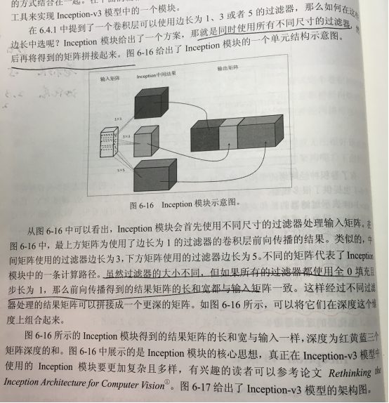
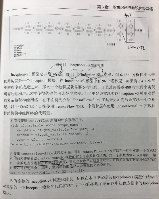
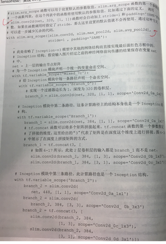
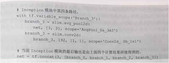
(2)Inception-v3 模型
slim子模块介绍:【Tensorflow】辅助工具篇——tensorflow slim(TF-Slim)介绍
6.5 卷积神经网络迁移学习
所谓迁移学习,就是将一个问题上训练好的模型通过简单的调整使其适用于一个新的问题。
根据论文DeCAF:A Deep Convolutional Activation Feature for Generic Visual Recognition中的结论,可以保留Inception-v3模型中所有卷积层的参数,只是替换最后一层全连接层。在最后这一层全连接层之前的网络层称之为瓶颈层(bottleneck)。
将新的图像通过训练好的卷积神经网络直到瓶颈层的过程可以看成是对图像进行特征提取的过程,瓶颈层输出的节点向量可以被作为任何图像的一个更加精简且表达能力更强的特征向量。
于是,在新数据集上,可以直接利用这个训练好的神经网络对图像进行特征提取,然后再将提取得到的特征向量作为输入来训练一个新的单层全连接神经网络处理新的分类问题。
#!/usr/bin/env python3

# -*- coding: utf-8 -*-


import glob

import os.path

import random

import numpy as np

import tensorflow as tf

from tensorflow.python.platform import gfile


# Inception-v3模型瓶颈层的节点个数

BOTTLENECK_TENSOR_SIZE = 2048


# Inception-v3模型中代表瓶颈层结果的张量名称。

# 在谷歌提出的Inception-v3模型中,这个张量名称就是'pool_3/_reshape:0'。

# 在训练模型时,可以通过tensor.name来获取张量的名称。

BOTTLENECK_TENSOR_NAME = 'pool_3/_reshape:0'


# 图像输入张量所对应的名称。

JPEG_DATA_TENSOR_NAME = 'DecodeJpeg/contents:0'


# 下载的谷歌训练好的Inception-v3模型文件目录

MODEL_DIR = 'model/'


# 下载的谷歌训练好的Inception-v3模型文件名

MODEL_FILE = 'tensorflow_inception_graph.pb'


# 因为一个训练数据会被使用多次,所以可以将原始图像通过Inception-v3模型计算得到的特征向量保存在文件中,免去重复的计算。

# 下面的变量定义了这些文件的存放地址。

CACHE_DIR = 'tmp/bottleneck/'


# 图片数据文件夹。

# 在这个文件夹中每一个子文件夹代表一个需要区分的类别,每个子文件夹中存放了对应类别的图片。

INPUT_DATA = 'flower_data/'


# 验证的数据百分比

VALIDATION_PERCENTAGE = 10

# 测试的数据百分比

TEST_PERCENTAGE = 10


# 定义神经网络的设置

LEARNING_RATE = 0.01

STEPS = 4000

BATCH = 100


# 这个函数从数据文件夹中读取所有的图片列表并按训练、验证、测试数据分开。

# testing_percentage和validation_percentage参数指定了测试数据集和验证数据集的大小。

def create_image_lists(testing_percentage, validation_percentage):

    # 得到的所有图片都存在result这个字典(dictionary)里。

    # 这个字典的key为类别的名称,value也是一个字典,字典里存储了所有的图片名称。

    result = {}

    # 获取当前目录下所有的子目录

    sub_dirs = [x[0] for x in os.walk(INPUT_DATA)]

    # 得到的第一个目录是当前目录,不需要考虑

    is_root_dir = True

    for sub_dir in sub_dirs:

        if is_root_dir:

            is_root_dir = False

            continue


        # 获取当前目录下所有的有效图片文件。

        extensions = ['jpg', 'jpeg', 'JPG', 'JPEG']

        file_list = []

        dir_name = os.path.basename(sub_dir)

        for extension in extensions:

            file_glob = os.path.join(INPUT_DATA, dir_name, '*.'+extension)

            file_list.extend(glob.glob(file_glob))

        if not file_list:

            continue


        # 通过目录名获取类别的名称。

        label_name = dir_name.lower()

        # 初始化当前类别的训练数据集、测试数据集和验证数据集

        training_images = []

        testing_images = []

        validation_images = []

        for file_name in file_list:

            base_name = os.path.basename(file_name)

            # 随机将数据分到训练数据集、测试数据集和验证数据集。

            chance = np.random.randint(100)

            if chance < validation_percentage:

                validation_images.append(base_name)

            elif chance < (testing_percentage + validation_percentage):

                testing_images.append(base_name)

            else:

                training_images.append(base_name)


        # 将当前类别的数据放入结果字典。

        result[label_name] = {

            'dir': dir_name,

            'training': training_images,

            'testing': testing_images,

            'validation': validation_images

            }

    # 返回整理好的所有数据

    return result


# 这个函数通过类别名称、所属数据集和图片编号获取一张图片的地址。

# image_lists参数给出了所有图片信息。

# image_dir参数给出了根目录。存放图片数据的根目录和存放图片特征向量的根目录地址不同。

# label_name参数给定了类别的名称。

# index参数给定了需要获取的图片的编号。

# category参数指定了需要获取的图片是在训练数据集、测试数据集还是验证数据集。

def get_image_path(image_lists, image_dir, label_name, index, category):

    # 获取给定类别中所有图片的信息。

    label_lists = image_lists[label_name]

    # 根据所属数据集的名称获取集合中的全部图片信息。

    category_list = label_lists[category]

    mod_index = index % len(category_list)

    # 获取图片的文件名。

    base_name = category_list[mod_index]

    sub_dir = label_lists['dir']

    # 最终的地址为数据根目录的地址 + 类别的文件夹 + 图片的名称

    full_path = os.path.join(image_dir, sub_dir, base_name)

    return full_path


# 这个函数通过类别名称、所属数据集和图片编号获取经过Inception-v3模型处理之后的特征向量文件地址。

def get_bottlenect_path(image_lists, label_name, index, category):

    return get_image_path(image_lists, CACHE_DIR, label_name, index, category) + '.txt';


# 这个函数使用加载的训练好的Inception-v3模型处理一张图片,得到这个图片的特征向量。

def run_bottleneck_on_image(sess, image_data, image_data_tensor, bottleneck_tensor):

    # 这个过程实际上就是将当前图片作为输入计算瓶颈张量的值。这个瓶颈张量的值就是这张图片的新的特征向量。

    bottleneck_values = sess.run(bottleneck_tensor, {image_data_tensor: image_data})

    # 经过卷积神经网络处理的结果是一个四维数组,需要将这个结果压缩成一个特征向量(一维数组)

    bottleneck_values = np.squeeze(bottleneck_values)

    return bottleneck_values


# 这个函数获取一张图片经过Inception-v3模型处理之后的特征向量。

# 这个函数会先试图寻找已经计算且保存下来的特征向量,如果找不到则先计算这个特征向量,然后保存到文件。

def get_or_create_bottleneck(sess, image_lists, label_name, index, category, jpeg_data_tensor, bottleneck_tensor):

    # 获取一张图片对应的特征向量文件的路径。

    label_lists = image_lists[label_name]

    sub_dir = label_lists['dir']

    sub_dir_path = os.path.join(CACHE_DIR, sub_dir)

    if not os.path.exists(sub_dir_path):

        os.makedirs(sub_dir_path)

    bottleneck_path = get_bottlenect_path(image_lists, label_name, index, category)

    # 如果这个特征向量文件不存在,则通过Inception-v3模型来计算特征向量,并将计算的结果存入文件。

    if not os.path.exists(bottleneck_path):

        # 获取原始的图片路径

        image_path = get_image_path(image_lists, INPUT_DATA, label_name, index, category)

        # 获取图片内容。

        image_data = gfile.FastGFile(image_path, 'rb').read()

        # print(len(image_data))

        # 由于输入的图片大小不一致,此处得到的image_data大小也不一致(已验证),但却都能通过加载的inception-v3模型生成一个2048的特征向量。具体原理不详。

        # 通过Inception-v3模型计算特征向量

        bottleneck_values = run_bottleneck_on_image(sess, image_data, jpeg_data_tensor, bottleneck_tensor)

        # 将计算得到的特征向量存入文件

        bottleneck_string = ','.join(str(x) for x in bottleneck_values)

        with open(bottleneck_path, 'w') as bottleneck_file:

            bottleneck_file.write(bottleneck_string)

    else:

        # 直接从文件中获取图片相应的特征向量。

        with open(bottleneck_path, 'r') as bottleneck_file:

            bottleneck_string = bottleneck_file.read()

        bottleneck_values = [float(x) for x in bottleneck_string.split(',')]

    # 返回得到的特征向量

    return bottleneck_values


# 这个函数随机获取一个batch的图片作为训练数据。

def get_random_cached_bottlenecks(sess, n_classes, image_lists, how_many, category,

                                  jpeg_data_tensor, bottleneck_tensor):

    bottlenecks = []

    ground_truths = []

    for _ in range(how_many):

        # 随机一个类别和图片的编号加入当前的训练数据。

        label_index = random.randrange(n_classes)

        label_name = list(image_lists.keys())[label_index]

        image_index = random.randrange(65536)

        bottleneck = get_or_create_bottleneck(sess, image_lists, label_name, image_index, category,

                                              jpeg_data_tensor, bottleneck_tensor)

        ground_truth = np.zeros(n_classes, dtype=np.float32)

        ground_truth[label_index] = 1.0

        bottlenecks.append(bottleneck)

        ground_truths.append(ground_truth)

    return bottlenecks, ground_truths


# 这个函数获取全部的测试数据。在最终测试的时候需要在所有的测试数据上计算正确率。

def get_test_bottlenecks(sess, image_lists, n_classes, jpeg_data_tensor, bottleneck_tensor):

    bottlenecks = []

    ground_truths = []

    label_name_list = list(image_lists.keys())

    # 枚举所有的类别和每个类别中的测试图片。

    for label_index, label_name in enumerate(label_name_list):

        category = 'testing'

        for index, unused_base_name in enumerate(image_lists[label_name][category]):

            # 通过Inception-v3模型计算图片对应的特征向量,并将其加入最终数据的列表。

            bottleneck = get_or_create_bottleneck(sess, image_lists, label_name, index, category,

                                                  jpeg_data_tensor, bottleneck_tensor)

            ground_truth = np.zeros(n_classes, dtype = np.float32)

            ground_truth[label_index] = 1.0

            bottlenecks.append(bottleneck)

            ground_truths.append(ground_truth)

    return bottlenecks, ground_truths


def main(_):

    # 读取所有图片。

    image_lists = create_image_lists(TEST_PERCENTAGE, VALIDATION_PERCENTAGE)

    n_classes = len(image_lists.keys())

    # 读取已经训练好的Inception-v3模型。

    # 谷歌训练好的模型保存在了GraphDef Protocol Buffer中,里面保存了每一个节点取值的计算方法以及变量的取值。

    # TensorFlow模型持久化的问题在第5章中有详细的介绍。

    with gfile.FastGFile(os.path.join(MODEL_DIR, MODEL_FILE), 'rb') as f:

        graph_def = tf.GraphDef()

        graph_def.ParseFromString(f.read())

    # 加载读取的Inception-v3模型,并返回数据输入所对应的张量以及计算瓶颈层结果所对应的张量。

    bottleneck_tensor, jpeg_data_tensor = tf.import_graph_def(graph_def, return_elements=[BOTTLENECK_TENSOR_NAME, JPEG_DATA_TENSOR_NAME])

    # 定义新的神经网络输入,这个输入就是新的图片经过Inception-v3模型前向传播到达瓶颈层时的结点取值。

    # 可以将这个过程类似的理解为一种特征提取。

    bottleneck_input = tf.placeholder(tf.float32, [None, BOTTLENECK_TENSOR_SIZE], name='BottleneckInputPlaceholder')

    # 定义新的标准答案输入

    ground_truth_input = tf.placeholder(tf.float32, [None, n_classes], name='GroundTruthInput')

    # 定义一层全连接层来解决新的图片分类问题。

    # 因为训练好的Inception-v3模型已经将原始的图片抽象为了更加容易分类的特征向量了,所以不需要再训练那么复杂的神经网络来完成这个新的分类任务。

    with tf.name_scope('final_training_ops'):

        weights = tf.Variable(tf.truncated_normal([BOTTLENECK_TENSOR_SIZE, n_classes], stddev=0.001))

        biases = tf.Variable(tf.zeros([n_classes]))

        logits = tf.matmul(bottleneck_input, weights) + biases

        final_tensor = tf.nn.softmax(logits)

    # 定义交叉熵损失函数

    cross_entropy = tf.nn.softmax_cross_entropy_with_logits(logits=logits, labels=ground_truth_input)

    cross_entropy_mean = tf.reduce_mean(cross_entropy)

    train_step = tf.train.GradientDescentOptimizer(LEARNING_RATE).minimize(cross_entropy_mean)

    # 计算正确率

    with tf.name_scope('evaluation'):

        correct_prediction = tf.equal(tf.argmax(final_tensor, 1), tf.argmax(ground_truth_input, 1))

        evaluation_step = tf.reduce_mean(tf.cast(correct_prediction, tf.float32))


    with tf.Session() as sess:

        tf.global_variables_initializer().run()

        # 训练过程

        for i in range(STEPS):

            # 每次获取一个batch的训练数据

            train_bottlenecks, train_ground_truth = get_random_cached_bottlenecks(

                sess, n_classes, image_lists, BATCH, 'training', jpeg_data_tensor, bottleneck_tensor)

            sess.run(train_step, feed_dict={bottleneck_input: train_bottlenecks, ground_truth_input: train_ground_truth})

            # 在验证集上测试正确率。

            if i%100 == 0 or i+1 == STEPS:

                validation_bottlenecks, validation_ground_truth = get_random_cached_bottlenecks(

                    sess, n_classes, image_lists, BATCH, 'validation', jpeg_data_tensor, bottleneck_tensor)

                validation_accuracy = sess.run(evaluation_step, feed_dict={

                    bottleneck_input:validation_bottlenecks, ground_truth_input: validation_ground_truth})

                print('Step %d: Validation accuracy on random sampled %d examples = %.1f%%'

                      % (i, BATCH, validation_accuracy*100))

        # 在最后的测试数据上测试正确率

        test_bottlenecks, test_ground_truth = get_test_bottlenecks(sess, image_lists, n_classes,

                                                                       jpeg_data_tensor, bottleneck_tensor)

        test_accuracy = sess.run(evaluation_step, feed_dict={bottleneck_input: test_bottlenecks,

                                                                 ground_truth_input: test_ground_truth})

        print('Final test accuracy = %.1f%%' % (test_accuracy * 100))


if __name__ == '__main__':

    tf.app.run()
1.4.0/Chapter06$ python2 transfer_flower.py
2018-03-13 22:54:12.743299: I tensorflow/core/platform/cpu_feature_guard.cc:137] Your CPU supports instructions that this TensorFlow binary was not compiled to use: SSE4.1 SSE4.2 AVX
2018-03-13 22:54:13.803336: W tensorflow/core/framework/op_def_util.cc:334] Op BatchNormWithGlobalNormalization is deprecated. It will cease to work in GraphDef version 9. Use tf.nn.batch_normalization().
Step 0: Validation accuracy on random sampled 100 examples = 39.0%
Step 100: Validation accuracy on random sampled 100 examples = 77.0%
Step 200: Validation accuracy on random sampled 100 examples = 84.0%
Step 300: Validation accuracy on random sampled 100 examples = 84.0%
Step 400: Validation accuracy on random sampled 100 examples = 89.0%
Step 500: Validation accuracy on random sampled 100 examples = 90.0%
Step 600: Validation accuracy on random sampled 100 examples = 93.0%
Step 700: Validation accuracy on random sampled 100 examples = 92.0%
Step 800: Validation accuracy on random sampled 100 examples = 91.0%
Step 900: Validation accuracy on random sampled 100 examples = 85.0%
Step 1000: Validation accuracy on random sampled 100 examples = 89.0%
Step 1100: Validation accuracy on random sampled 100 examples = 88.0%
Step 1200: Validation accuracy on random sampled 100 examples = 92.0%
Step 1300: Validation accuracy on random sampled 100 examples = 90.0%
Step 1400: Validation accuracy on random sampled 100 examples = 90.0%
Step 1500: Validation accuracy on random sampled 100 examples = 91.0%
Step 1600: Validation accuracy on random sampled 100 examples = 92.0%
Step 1700: Validation accuracy on random sampled 100 examples = 92.0%
Step 1800: Validation accuracy on random sampled 100 examples = 88.0%
Step 1900: Validation accuracy on random sampled 100 examples = 93.0%
Step 2000: Validation accuracy on random sampled 100 examples = 83.0%
Step 2100: Validation accuracy on random sampled 100 examples = 88.0%
Step 2200: Validation accuracy on random sampled 100 examples = 94.0%
Step 2300: Validation accuracy on random sampled 100 examples = 92.0%
Step 2400: Validation accuracy on random sampled 100 examples = 94.0%
Step 2500: Validation accuracy on random sampled 100 examples = 93.0%
Step 2600: Validation accuracy on random sampled 100 examples = 88.0%
Step 2700: Validation accuracy on random sampled 100 examples = 94.0%
Step 2800: Validation accuracy on random sampled 100 examples = 93.0%
Step 2900: Validation accuracy on random sampled 100 examples = 89.0%
Step 3000: Validation accuracy on random sampled 100 examples = 88.0%
Step 3100: Validation accuracy on random sampled 100 examples = 93.0%
Step 3200: Validation accuracy on random sampled 100 examples = 88.0%
Step 3300: Validation accuracy on random sampled 100 examples = 87.0%
Step 3400: Validation accuracy on random sampled 100 examples = 87.0%
Step 3500: Validation accuracy on random sampled 100 examples = 92.0%
Step 3600: Validation accuracy on random sampled 100 examples = 93.0%
Step 3700: Validation accuracy on random sampled 100 examples = 89.0%
Step 3800: Validation accuracy on random sampled 100 examples = 92.0%
Step 3900: Validation accuracy on random sampled 100 examples = 96.0%
Step 3999: Validation accuracy on random sampled 100 examples = 87.0%
Final test accuracy = 92.9%
原理:在训练好的inception-v3模型中,因为将瓶颈层的输出再通过一个单层的全连接层神经网络可以很好的区分1000种类别的图像,所以可以认为瓶颈层输出的节点向量可以被作为任何图像的一个更具有表达能力的特征向量。于是在新的数据集上可以直接利用这个训练好的神经网络对图像进行特征提取,然后将提取得到的特征向量作为输入来训练一个全新的单层全连接神经网络处理新的分类问题。
一般来说在数据量足够的情况下,迁移学习的效果不如完全重新训练。但是迁移学习所需要的训练时间和训练样本要远远小于训练完整的模型。