Contents
Introduction
天池比赛项目,作为练习,这是第一个版本。赛题内容如下:
商家有时会在特定日期(例如“Boxing-day” ,“ 黑色星期五” 或“ 双11” )进行大促销(例如折扣或现金券),以吸引大量新买家。许多吸引的买家都是一次性交易猎人,这些促销可能对销售产生很小的长期影响。为了缓解这个问题,商家必须确定谁可以转换为重复买家。通过瞄准这些潜力忠诚的客户,商家可以大大降低促销成本,提高投资回报率(ROI )。
众所周知,在线广告领域,客户定位极具挑战性,特别是对于新买家而言。但是通过Tmall.com 长期积累的用户行为日志,我们或许可以解决这个问题。在这个挑战中,我们提供了一套商家及其在“双11 ”日促销期间获得的相应新买家。你的任务是预测对于指定商家的新买家将来是否会成为忠实客户。换句话说,您需要预测这些新买家在6 个月内再次从同一商家购买商品的概率。一个包含大约20 万用户的数据集用于训练,还有一个类似大小的数据集用于测试。与其他比赛类似,您可以提取任何特征,然后使用其他工具进行训练。您只需提交预测结果进行评估。
EDA
./data_format1/中
- train_format1.csv提供了训练数据的(用户id, 商家id, 标签);
- test_format1.csv提供了测试数据的(用户id, 商家id);
- user_info_format1.csv提供了所有用户的年龄和性别信息;
- user_log_format1.csv提供了所有用户的行为,包括:
- 用户id, 商家id,
- 该用户在该商家所感兴趣的:
- 商品id, 类别id, 品牌id, 行为日期(time_stamp),行为类别(包括0点击,1加入购物车,2购买,3收藏该店铺)
./data_format2/中包括的信息是一样的,但表达形式不同
- train_format2.csv中的标签有-1,0,1,除了1之外,这里的-1表示该条数据不作为训练数据使用,但也记录了用户的行为,这些数据都被整合在了user_log_format1.csv中
特征组合
import pandas as pd
import numpy as np
train_feature = pd.read_csv('./traindata_features.csv')
features = list(train_feature.columns[3:])
print(features)
['num_action0', 'num_action1', 'num_action2', 'num_action3', 'ttl_items', 'ttl_cats', 'ttl_brands', 'bought_item_types', 'bought_cat_types', 'bought_brand_types', 'addtocart', 'addtofavorite', 'age__0.0', 'age__1.0', 'age__2.0', 'age__3.0', 'age__4.0', 'age__5.0', 'age__6.0', 'age__7.0', 'age__8.0', 'gender__0.0', 'gender__1.0', 'gender__2.0', 'ttlnum_item_types_in', 'ttlnum_cat_types_in', 'ttlnum_brand_types_in', 'ttlnum_item_types_all', 'ttlnum_cat_types_all', 'num_action0_in', 'num_action1_in', 'num_action2_in', 'num_buyers_in', 'num_buyers_buymore_in', 'num_action0_userin', 'num_action1_userin', 'num_action2_userin', 'num_action3_userin', 'num_action0_userall', 'num_action1_userall', 'num_action2_userall', 'num_action3_userall', 'num_items', 'item_boughtFreq_old', 'item_boughtFreq_new', 'item_boughtFreq_all', 'cat_boughtFreq_old', 'cat_boughtFreq_new', 'cat_boughtFreq_all', 'brand_boughtFreq_old', 'brand_boughtFreq_new', 'brand_boughtFreq_all', 'usr_buy_days', 'num_repeatbuy', '30days_repeatusers_cnt_max', '30days_repeatusers_cnt_min', '30days_repeatusers_cnt_avg', '60days_repeatusers_cnt_max', '60days_repeatusers_cnt_min', '60days_repeatusers_cnt_avg', '90days_repeatusers_cnt_max', '90days_repeatusers_cnt_min', '90days_repeatusers_cnt_avg']
len(features)
63
对于每一对(用户, 商家),得到特征:
- (uid, sid): #(点击数), #(加入购物车数), #(购买数), #(收藏数).
- (uid, sid): #(涵盖商品数目), #(涵盖商品类别), #(涵盖品牌).
- (uid, sid): #(购买的商品数目), #(购买的商品类别), #(购买的品牌数目).
- (uid, sid): ?(是否加入购物车), ?(是否收藏)
对于每一个(商家),得到特征:
- 训练集中出现的:商品种类总数,类别种类总数,品牌种类总数;
- 用户日志中出现过的:商品种类总数,类别种类总数,品牌种类总数。
- 训练集中出现的:点击总数,加入购物车总数,购买总数,收藏总数;
- 用户日志中出现过的:点击总数,加入购物车总数,购买总数,收藏总数.
- 训练集中出现过的:买家总数,购买次数2次或以上的买家总数;
- 用户日志中出现过的:买家总数,购买次数2次或以上的买家总数。
通过相关性分析,我们只保留相关系数小于0.9的特征组合:
- 训练集中出现的:商商品种类总数,类别种类总数,品牌种类总数;
- 用户日志中出现过的:商商品种类总数,类别种类总数,品牌种类总数。
- 训练集中出现的:点击总数,加入购物车总数,购买总数。
- 训练集中出现过的:买家总数,购买次数2次或以上的买家总数.
对于每一个(用户),得到特征:
- 年龄,性别,进行独热向量编码。
- 训练集中出现的:点击总数,加入购物车总数,购买总数,收藏总数;
- 用户日志中出现过的:点击总数,加入购物车总数,购买总数,收藏总数.
通过相关性分析,以上特征相关系数均小于0.9,因此都保留了。
针对购买的商品,可以提取以下特征:
- 对训练集/测试集中的每一对(用户,商家),计算
- num_items: 购买商品次数。
- item_boughtFreq_old:所购买的商品在用户日志中(label=-1)被购买的频率,取最大值(还可以加入最小值、标准差,但是实验的时候忘记了);
- item_boughtFreq_new: 所购买的商品在新增样本中(label=0,1)被购买的频率,取最大值;
- item_boughtFreq_all: 所购买的商品在全部样本中(label=-1,0,1)被购买的频率,取最大值;
- 上述三个特征分别应用于所购买的商品类别和品牌,又可以得到6个特征: 'cat_boughtFreq_old', 'cat_boughtFreq_new', 'cat_boughtFreq_all', 'brand_boughtFreq_old', 'brand_boughtFreq_new', 'brand_boughtFreq_all'.
利用时间戳提取特征:
- 用户有购买行为的天数;
- 一个用户重复购买的次数。
- 对于一对(用户、商家):统计30天,60天,90天,类别被购买次数的最大、最小、标准差,可以看是否为常用各类别。
目前为止,得到共计63个特征。
缺失值处理
在该数据集中,存在缺失值的有年龄、性别、品牌。因年龄和性别的确实比例很少(1%左右),我们使用众数填充。
对于品牌id,可以根据其关联的商品和类别进行填充,从相同(用户,商品、类别、商家,时间戳)开始找,逐渐减少对照列,直到找到非空集合,使用众数填充。
def fill_brand_id_nan(datalog):
    ix_group = datalog[datalog.brand_id.isnull()].ix[:, ['user_id','seller_id','cat_id', 'item_id', 'time_stamp']]
    ix_nan = [{'uid': x[1].user_id, 'sid': x[1].seller_id, 'cid':x[1].cat_id, 'tid': x[1].item_id, 'time':x[1].time_stamp} for x in ix_group.iterrows()]

    tmp1 = datalog.groupby(['user_id', 'seller_id','cat_id', 'item_id', 'time_stamp'])
    tmp2 = datalog.groupby(['user_id', 'seller_id', 'cat_id', 'item_id'])
    tmp3 = datalog.groupby(['seller_id', 'cat_id'])
    tmp4 = datalog.groupby(['seller_id', 'item_id'])
    tmp5 = datalog.groupby(['seller_id'])

    replace_value = []
    for xindex, x in ix_group.iterrows():
        rv = tmp1.get_group((x.user_id, x.seller_id, x.cat_id, x.item_id, x.time_stamp)).brand_id.mode()
        if rv.empty:
            rv = tmp2.get_group((x.user_id, x.seller_id, x.cat_id, x.item_id)).brand_id.mode()
            if rv.empty:
                rv = tmp3.get_group((x.seller_id, x.cat_id)).brand_id.mode()
                if rv.empty:
                    rv = tmp4.get_group((x.seller_id, x.item_id)).brand_id.mode()
                    if rv.empty:
                        rv = tmp5.get_group((x.seller_id)).brand_id.mode()
        try:
            replace_value.append(rv)
            datalog.brand_id[xindex] = rv[0]
        except:
            print('Error')
            print(tmp1.get_group((x.user_id, x.seller_id, x.cat_id, x.item_id, x.time_stamp)))
            print(tmp2.get_group((x.user_id, x.seller_id, x.cat_id, x.item_id)))
            break

    return datalog
对特征进行归一化/标准化处理:
from sklearn.preprocessing import MinMaxScaler,StandardScaler

x = train_feature[features]

minmax = MinMaxScaler()
minmax.fit(x.as_matrix())
x_mm = minmax.transform(x.as_matrix())
x_mm = pd.DataFrame(x_mm, columns = x.columns)

scaler = StandardScaler()
scaler.fit(x.as_matrix())
x_scal = scaler.transform(x.as_matrix())
x_scal = pd.DataFrame(x_scal, columns = x.columns)
from sklearn.model_selection import train_test_split
y = train_feature['label']
X_train, X_test, y_train, y_test = train_test_split(x_mm[features].values, y.values, test_size=0.25)
特征重要性
from sklearn.externals import joblib
clf_xgb = joblib.load('./model/model_xgb_X_train_feat63_0.6849504_583rounds.m')

from xgboost import plot_importance
from matplotlib import pyplot as plt
%matplotlib inline
fig,axes = plt.subplots(figsize=(10,15))
plot_importance(clf_xgb,ax=axes)

featdict = dict(zip(clf_xgb.feature_names,features))
yticklabel = [d.get_text() for d in list(axes.get_yticklabels())]
toset_yticklabel = [featdict[y]for y in yticklabel]

axes.set_yticklabels(toset_yticklabel)
# axes.get_yticklabels
plt.show()
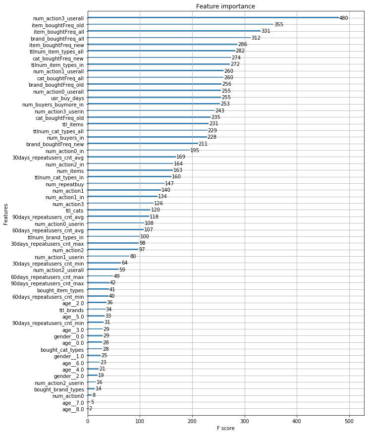
可以看出,重要度排在前面的有:
- 对于每一个(用户),用户日志中出现过的收藏总数;
- 对于每一对(用户,商家),所购买的商品在用户日志中(label=-1)被购买的频率的最大值;
- 对于每一对(用户,商家),所购买的商品在全部样本中(label=-1,0,1)被购买的频率的最大值;
- 对于每一对(用户,商家),所购买的品牌在全部样本中(label=-1,0,1)被购买的频率的最大值;
- 对于每一对(用户,商家),所购买的商品在新增样本中(label=0,1)被购买的频率的最大值;
- 对于每一个(商家),用户日志中出现过的商品种类总数;
- 对于每一对(用户,商家),所购买的类别在新增样本中(label=0,1)被购买的频率的最大值;
- 对于每一个(商家),训练集样本中出现过的商品种类总数。
- 对于每一个(用户),用户日志中出现过的加入购物车总数;
- 对于每一对(用户,商家),所购买的类别在全部样本中(label=-1,0,1)被购买的频率的最大值;
- 对于每一对(用户,商家),所购买的品牌在用户日志中(label=-1)被购买的频率的最大值;
- 对于每一个(用户), 用户日志中出现过的点击总数;
...
如果调整num_boost_round, 会使特征重要度排名稍微改变,但总体变化并不大。
该模型的训练过程如下:
xgb_params = {
    # general parameters
    'booster': 'gbtree',
    'silent': 1,

    # booster parameters
    'learning_rate': 0.05,
    'gamma': 0,
    'max_depth': 4,
    'min_child_weight': 1,
    'max_delta_step': 0,
    'subsample': 0.5,
    'colsample_bytree': 1.0,

    # task parameters
    'objective': 'reg:logistic',
    'eval_metric': 'auc',
    'seed': 0,
}
x = train_feature[features]
y = train_feature['label']
X_train, X_test, y_train, y_test = train_test_split(x,y, test_size=0.25) #data is split in a stratified fashion
dtrain = xgb.DMatrix(X_train[features].values,y_train['label'].values)
clf_xgb = xgb.train(xgb_params, dtrain=dtrain, num_boost_round = 583)

# num_boost_round = 583:
#       用相同的参数跑了交叉验证(xgb.cv),cv_num=5,在第583轮的时候测试集平均auc最高。
#data is split in a stratified fashion
joblib.dump(toset_yticklabel,'./model/feat_importance1.m')
['./model/feat_importance1.m']
Different Machine Learning Models
XGBoost
import xgboost as xgb
njobs = 2
xgb1 = xgb.XGBClassifier(scale_pos_weight = 15.3,
                         n_estimators = 600,
                         learning_rate = 0.05,
                         max_depth = 4,
                         min_child_weight = 1,
                         subsample = 0.5,
                         gamma = 0,
                         colsample_bytree = 1,
                         objective = 'reg:logistic',
                         eval_metric = 'auc',
                         seed = 0,
                         nthread = njobs)
xgb1.fit(X_train, y_train)
probas_xgb = xgb1.predict_proba(X_test)
pred_xgb = xgb1.predict(X_test)


from sklearn.metrics import roc_auc_score
# y_test = y_test.tolist()
auc_xgb = roc_auc_score(y_test, pred_xgb)
D:UsersgaoAnaconda3libsite-packagessklearnpreprocessinglabel.py:151: DeprecationWarning: The truth value of an empty array is ambiguous. Returning False, but in future this will result in an error. Use `array.size > 0` to check that an array is not empty.
  if diff:
Random Forest
from sklearn.ensemble import RandomForestClassifier
njobs = 2
rf1 = RandomForestClassifier(class_weight={0: 1, 1: 15.3},
                             criterion = 'gini',
                             max_depth = 50,
                             max_features = 'sqrt',
                             max_leaf_nodes = None,
                             min_samples_leaf = 20,
                             min_samples_split = 50,
                             n_estimators = 750,
                             random_state = 0)
rf1.fit(X_train, y_train)
probas_rf = rf1.predict_proba(X_test)
pred_rf = rf1.predict(X_test)


from sklearn.metrics import roc_auc_score
# y_test = y_test.tolist()
auc_rf = roc_auc_score(y_test, pred_rf)
GBDT
from sklearn.ensemble import GradientBoostingClassifier
njobs = 2
gbdt1 = GradientBoostingClassifier(learning_rate = 0.05,
                                  subsample = 0.5,
                                  max_depth = 5,
                                  n_estimators = 100,
                                  loss = 'deviance',
                                  random_state = 0,
                                  min_samples_split = 100,
                                  min_samples_leaf = 120,
                                  max_features = 'sqrt',
                                  )

gbdt1.fit(X_train, y_train)
probas_gbdt = gbdt1.predict_proba(X_test)
pred_gbdt = gbdt1.predict(X_test)


from sklearn.metrics import roc_auc_score
# y_test = y_test.tolist()
auc_gbdt = roc_auc_score(y_test, pred_gbdt)
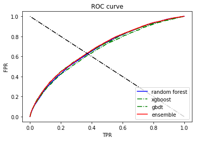
Plot ROC Curve
from sklearn.metrics import roc_curve, auc
import matplotlib.pyplot as plt
import numpy as np

fpr, tpr, thresholds = roc_curve(y_test, probas_rf[:, 1])
roc_auc = auc(fpr, tpr)
print('rf AUC:', roc_auc)
plt.plot(fpr, tpr, 'b-', label = 'random forest')

fpr, tpr, thresholds = roc_curve(y_test, probas_xgb[:, 1])
roc_auc = auc(fpr, tpr)
print('xgb AUC:', roc_auc)
plt.plot(fpr, tpr, 'g-.', label= 'xgboost')

fpr, tpr, thresholds = roc_curve(y_test, probas_gbdt[:, 1])
roc_auc = auc(fpr, tpr)
print('gbdt AUC:', roc_auc)
plt.plot(fpr, tpr, 'g-.', label= 'gbdt')

score_all = (np.array(probas_rf[:, 1]) + np.array(probas_xgb[:, 1]) + np.array(probas_gbdt[:, 1]))*0.5
fpr, tpr, thresholds = roc_curve(y_test, score_all)
roc_auc = auc(fpr, tpr)
print('AUC:', roc_auc)
plt.plot(fpr, tpr, 'r', label = 'ensemble')

plt.plot([1,0],[0,1], 'k-.')

plt.ylabel('FPR')
plt.xlabel('TPR')
plt.title('ROC curve')
plt.legend(loc="lower right")

# plt.savefig('ROC.png', dpi =1000)
rf AUC: 0.6796455895487219
xgb AUC: 0.6828011772216968
gbdt AUC: 0.6670128952067169
AUC: 0.6861724266190854


<matplotlib.legend.Legend at 0x2a816cca898>
调参
def train_optimal_classifier(clf,param,xdata,ydata):
    grid_search = GridSearchCV(
        clf,
        param_grid=param,
        cv=cv_num,
        verbose=2,
        scoring='roc_auc',
        error_score=0,
        refit=True ,
        n_jobs=njobs
        )

    grid_search.fit(xdata, ydata)
    print("Best parameters")
    print(grid_search.best_params_)
    print('best auc: ')
    print(grid_search.best_score_)
    return (grid_search.best_estimator_)
Model Blending by Stacking
将train data划分后,在训练集上交叉验证+模型融合(xgboost->random forest->GBDT),在测试集上预测结果:
clfs = [xgb1, rf1, gbdt1]

X_train, X_test, y_train, y_test = train_test_split(x_mm[features].values, y.values, test_size=0.25)
dataset_blend_train = np.zeros((X_train.shape[0], len(clfs)))
dataset_blend_test = np.zeros((X_test.shape[0], len(clfs)))
# '''5fold stacking'''
n_folds = 5
skf = list(StratifiedKFold(y_train, n_folds))
for j, clf in enumerate(clfs):
#    '''依次训练各个单模型'''
    print(j, clf)

    dataset_blend_test_j = np.zeros((X_test.shape[0], len(skf)))

    for i, (train, test) in enumerate(skf):
#        '''使用第i个部分作为预测,剩余的部分来训练模型,获得其预测的输出作为第i部分的新特征。'''
        print("Fold", i)
        X_ttrain, y_ttrain, X_ttest, y_ttest = X_train[train], y_train[train], X_train[test], y_train[test]
        clf.fit(X_ttrain, y_ttrain)
        y_submission = clf.predict_proba(X_ttest)[:, 1]
        dataset_blend_train[test, j] = y_submission
        dataset_blend_test_j[:, i] = clf.predict_proba(X_test)[:, 1]
#    '''对于测试集,直接用这k个模型的预测值均值作为新的特征。'''
    dataset_blend_test[:, j] = dataset_blend_test_j.mean(1)
    print("val auc Score: %f" % roc_auc_score(y_test, dataset_blend_test[:, j]))


# clf = LogisticRegression()
clf = GradientBoostingClassifier(learning_rate=0.02, subsample=0.5, max_depth=6, n_estimators=30)
clf.fit(dataset_blend_train, y_train)
y_submission = clf.predict_proba(dataset_blend_test)[:, 1]

print("Linear stretch of predictions to [0,1]")
y_submission = (y_submission - y_submission.min()) / (y_submission.max() - y_submission.min())
print("blend result")
print("val auc Score: %f" % (roc_auc_score(y_test, y_submission)))
一次运行后的输出如下,比相同参数下的各个模型单独训练的结果要好,进行模型融合auc后也有所提升:
0 XGBClassifier(base_score=0.5, booster='gbtree', colsample_bylevel=1,
colsample_bytree=1, eval_metric='auc', gamma=0, learning_rate=0.05,
max_delta_step=0, max_depth=4, min_child_weight=1, missing=None,
n_estimators=600, n_jobs=1, nthread=30, objective='reg:logistic',
random_state=0, reg_alpha=0, reg_lambda=1, scale_pos_weight=15.3,
seed=0, silent=True, subsample=0.5)
Fold 0
Fold 1
Fold 2
Fold 3
Fold 4
val auc Score: 0.689373
1 RandomForestClassifier(bootstrap=True, class_weight={0: 1, 1: 15.3},
criterion='gini', max_depth=50, max_features='sqrt',
max_leaf_nodes=None, min_impurity_decrease=0.0,
min_impurity_split=None, min_samples_leaf=20,
min_samples_split=50, min_weight_fraction_leaf=0.0,
n_estimators=750, n_jobs=30, oob_score=False, random_state=0,
verbose=0, warm_start=False)
Fold 0
Fold 1
Fold 2
Fold 3
Fold 4
val auc Score: 0.685798
2 GradientBoostingClassifier(criterion='friedman_mse', init=None,
learning_rate=0.05, loss='deviance', max_depth=5,
max_features='sqrt', max_leaf_nodes=None,
min_impurity_decrease=0.0, min_impurity_split=None,
min_samples_leaf=120, min_samples_split=100,
min_weight_fraction_leaf=0.0, n_estimators=100,
presort='auto', random_state=0, subsample=0.5, verbose=0,
warm_start=False)
Fold 0
Fold 1
Fold 2
Fold 3
Fold 4
val auc Score: 0.673720
Linear stretch of predictions to [0,1]
blend result
val auc Score: 0.692262
Summary
Reference
- 基于阿里巴巴大数据重复购买预测的实证研究, 王克利, 邓飞其,http://www.cnki.com.cn/Article/CJFDTotal-YNJR201803154.htm
- Ensemble Learning-模型融合-Python实现 by 立刻有, https://blog.csdn.net/shine19930820/article/details/75209021#3-python实现