TensorFlow(十)：卷积神经网络实现手写数字识别以及可视化

上代码：

import tensorflow as tf
from tensorflow.examples.tutorials.mnist import input_data

mnist = input_data.read_data_sets('MNIST_data',one_hot=True)

#每个批次的大小
batch_size = 100
#计算一共有多少个批次
n_batch = mnist.train.num_examples // batch_size

#参数概要
def variable_summaries(var):
    with tf.name_scope('summaries'):
        mean = tf.reduce_mean(var)
        tf.summary.scalar('mean', mean)#平均值
        with tf.name_scope('stddev'):
            stddev = tf.sqrt(tf.reduce_mean(tf.square(var - mean)))
        tf.summary.scalar('stddev', stddev)#标准差
        tf.summary.scalar('max', tf.reduce_max(var))#最大值
        tf.summary.scalar('min', tf.reduce_min(var))#最小值
        tf.summary.histogram('histogram', var)#直方图

#初始化权值
def weight_variable(shape,name):
    initial = tf.truncated_normal(shape,stddev=0.1)#生成一个截断的正态分布
    return tf.Variable(initial,name=name)

#初始化偏置
def bias_variable(shape,name):
    initial = tf.constant(0.1,shape=shape)
    return tf.Variable(initial,name=name)

#卷积层
def conv2d(x,W):
    #x input tensor of shape `[batch, in_height, in_width, in_channels]`
    #W filter / kernel tensor of shape [filter_height, filter_width, in_channels, out_channels]
    #`strides[0] = strides[3] = 1`. strides[1]代表x方向的步长，strides[2]代表y方向的步长
    #padding: A `string` from: `"SAME", "VALID"`
    return tf.nn.conv2d(x,W,strides=[1,1,1,1],padding='SAME')

#池化层
def max_pool_2x2(x):
    #ksize [1,x,y,1]
    return tf.nn.max_pool(x,ksize=[1,2,2,1],strides=[1,2,2,1],padding='SAME')

#命名空间
with tf.name_scope('input'):
    #定义两个placeholder
    x = tf.placeholder(tf.float32,[None,784],name='x-input')
    y = tf.placeholder(tf.float32,[None,10],name='y-input')
    with tf.name_scope('x_image'):
        #改变x的格式转为4D的向量[batch, in_height, in_width, in_channels]`
        x_image = tf.reshape(x,[-1,28,28,1],name='x_image')


with tf.name_scope('Conv1'):
    #初始化第一个卷积层的权值和偏置
    with tf.name_scope('W_conv1'):
        W_conv1 = weight_variable([5,5,1,32],name='W_conv1')#5*5的采样窗口，32个卷积核从1个平面抽取特征
    with tf.name_scope('b_conv1'):  
        b_conv1 = bias_variable([32],name='b_conv1')#每一个卷积核一个偏置值

    #把x_image和权值向量进行卷积，再加上偏置值，然后应用于relu激活函数
    with tf.name_scope('conv2d_1'):
        conv2d_1 = conv2d(x_image,W_conv1) + b_conv1
    with tf.name_scope('relu'):
        h_conv1 = tf.nn.relu(conv2d_1)
    with tf.name_scope('h_pool1'):
        h_pool1 = max_pool_2x2(h_conv1)#进行max-pooling

with tf.name_scope('Conv2'):
    #初始化第二个卷积层的权值和偏置
    with tf.name_scope('W_conv2'):
        W_conv2 = weight_variable([5,5,32,64],name='W_conv2')#5*5的采样窗口，64个卷积核从32个平面抽取特征
    with tf.name_scope('b_conv2'):  
        b_conv2 = bias_variable([64],name='b_conv2')#每一个卷积核一个偏置值

    #把h_pool1和权值向量进行卷积，再加上偏置值，然后应用于relu激活函数
    with tf.name_scope('conv2d_2'):
        conv2d_2 = conv2d(h_pool1,W_conv2) + b_conv2
    with tf.name_scope('relu'):
        h_conv2 = tf.nn.relu(conv2d_2)
    with tf.name_scope('h_pool2'):
        h_pool2 = max_pool_2x2(h_conv2)#进行max-pooling

#28*28的图片第一次卷积后还是28*28，第一次池化后变为14*14
#第二次卷积后为14*14，第二次池化后变为了7*7
#进过上面操作后得到64张7*7的平面

with tf.name_scope('fc1'):
    #初始化第一个全连接层的权值
    with tf.name_scope('W_fc1'):
        W_fc1 = weight_variable([7*7*64,1024],name='W_fc1')#上一场有7*7*64个神经元，全连接层有1024个神经元
    with tf.name_scope('b_fc1'):
        b_fc1 = bias_variable([1024],name='b_fc1')#1024个节点

    #把池化层2的输出扁平化为1维
    with tf.name_scope('h_pool2_flat'):
        h_pool2_flat = tf.reshape(h_pool2,[-1,7*7*64],name='h_pool2_flat')
    #求第一个全连接层的输出
    with tf.name_scope('wx_plus_b1'):
        wx_plus_b1 = tf.matmul(h_pool2_flat,W_fc1) + b_fc1
    with tf.name_scope('relu'):
        h_fc1 = tf.nn.relu(wx_plus_b1)

    #keep_prob用来表示神经元的输出概率
    with tf.name_scope('keep_prob'):
        keep_prob = tf.placeholder(tf.float32,name='keep_prob')
    with tf.name_scope('h_fc1_drop'):
        h_fc1_drop = tf.nn.dropout(h_fc1,keep_prob,name='h_fc1_drop')

with tf.name_scope('fc2'):
    #初始化第二个全连接层
    with tf.name_scope('W_fc2'):
        W_fc2 = weight_variable([1024,10],name='W_fc2')
    with tf.name_scope('b_fc2'):    
        b_fc2 = bias_variable([10],name='b_fc2')
    with tf.name_scope('wx_plus_b2'):
        wx_plus_b2 = tf.matmul(h_fc1_drop,W_fc2) + b_fc2
    with tf.name_scope('softmax'):
        #计算输出
        prediction = tf.nn.softmax(wx_plus_b2)

#交叉熵代价函数
with tf.name_scope('cross_entropy'):
    cross_entropy = tf.reduce_mean(tf.nn.softmax_cross_entropy_with_logits_v2(labels=y,logits=prediction),name='cross_entropy')
    tf.summary.scalar('cross_entropy',cross_entropy)
    
#使用AdamOptimizer进行优化
with tf.name_scope('train'):
    train_step = tf.train.AdamOptimizer(1e-4).minimize(cross_entropy)

#求准确率
with tf.name_scope('accuracy'):
    with tf.name_scope('correct_prediction'):
        #结果存放在一个布尔列表中
        correct_prediction = tf.equal(tf.argmax(prediction,1),tf.argmax(y,1))#argmax返回一维张量中最大的值所在的位置
    with tf.name_scope('accuracy'):
        #求准确率
        accuracy = tf.reduce_mean(tf.cast(correct_prediction,tf.float32))
        tf.summary.scalar('accuracy',accuracy)
        
#合并所有的summary
merged = tf.summary.merge_all()

with tf.Session() as sess:
    sess.run(tf.global_variables_initializer())
    train_writer = tf.summary.FileWriter('logs/train',sess.graph)
    test_writer = tf.summary.FileWriter('logs/test',sess.graph)
    for i in range(1001):
        #训练模型
        batch_xs,batch_ys =  mnist.train.next_batch(batch_size)
        sess.run(train_step,feed_dict={x:batch_xs,y:batch_ys,keep_prob:0.5})
        #记录训练集计算的参数
        summary = sess.run(merged,feed_dict={x:batch_xs,y:batch_ys,keep_prob:1.0})
        train_writer.add_summary(summary,i)
        #记录测试集计算的参数
        batch_xs,batch_ys =  mnist.test.next_batch(batch_size)
        summary = sess.run(merged,feed_dict={x:batch_xs,y:batch_ys,keep_prob:1.0})
        test_writer.add_summary(summary,i)
    
        if i%100==0:
            test_acc = sess.run(accuracy,feed_dict={x:mnist.test.images,y:mnist.test.labels,keep_prob:1.0})
            train_acc = sess.run(accuracy,feed_dict={x:mnist.train.images[:10000],y:mnist.train.labels[:10000],keep_prob:1.0})
            print ("Iter " + str(i) + ", Testing Accuracy= " + str(test_acc) + ", Training Accuracy= " + str(train_acc))

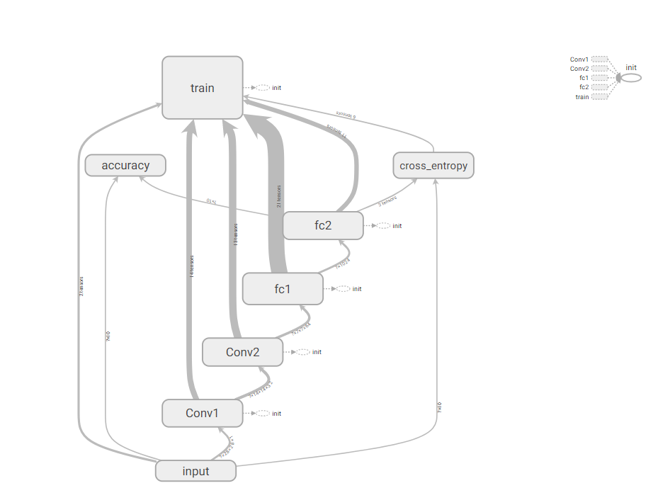
打开cmd，进入当前文件夹，执行tensorboard --logdir='C:UsersFELIXDesktop ensor学习logs'

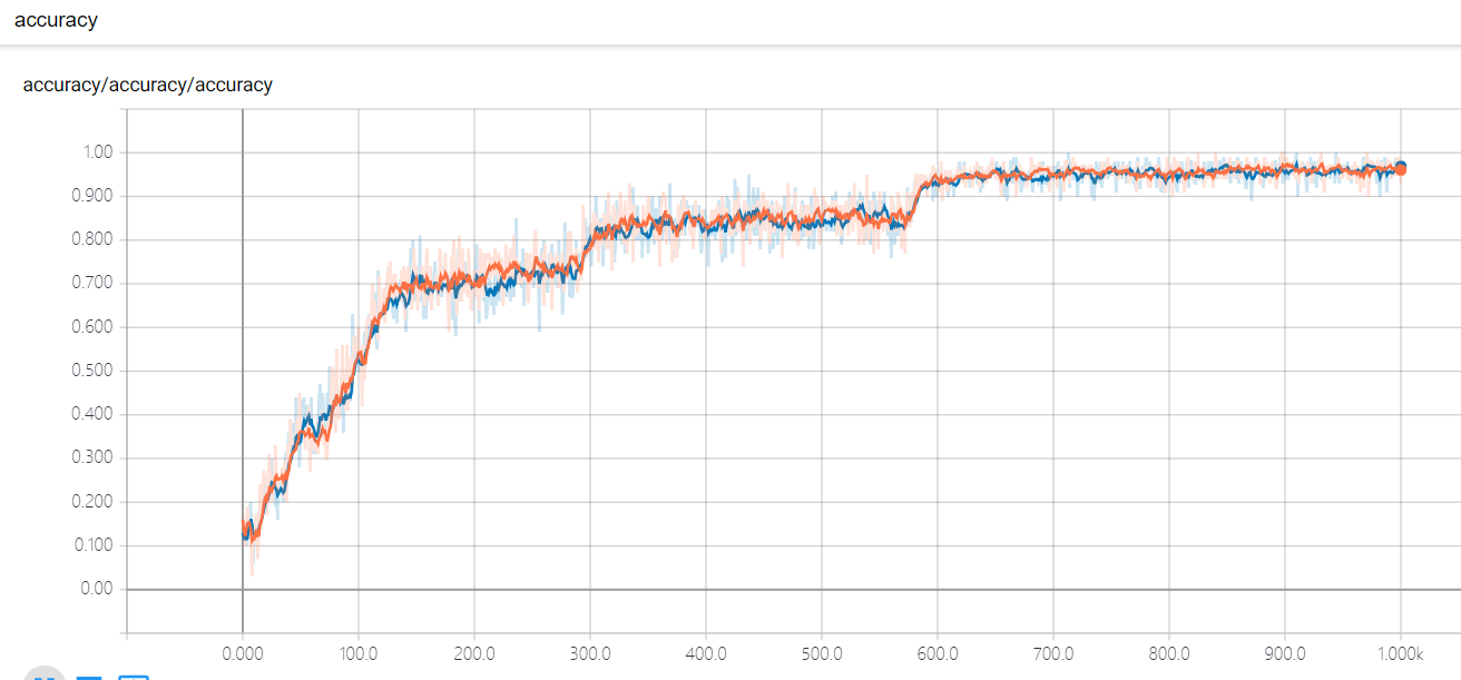
就可以进入tensorboard可视化界面了。