http://www.musicdsp.org/files/Audio-EQ-Cookbook.txt
https://arachnoid.com/BiQuadDesigner/index.html
https://blog.csdn.net/hunterhuang2013/article/details/64443718
Cookbook formulae for audio EQ biquad filter coefficients
----------------------------------------------------------------------------
by Robert Bristow-Johnson <rbj@audioimagination.com>
All filter transfer functions were derived from analog prototypes (that
are shown below for each EQ filter type) and had been digitized using the
Bilinear Transform. BLT frequency warping has been taken into account for
both significant frequency relocation (this is the normal "prewarping" that
is necessary when using the BLT) and for bandwidth readjustment (since the
bandwidth is compressed when mapped from analog to digital using the BLT).
First, given a biquad transfer function defined as:
b0 + b1*z^-1 + b2*z^-2
H(z) = ------------------------ (Eq 1)
a0 + a1*z^-1 + a2*z^-2
This shows 6 coefficients instead of 5 so, depending on your architechture,
you will likely normalize a0 to be 1 and perhaps also b0 to 1 (and collect
that into an overall gain coefficient). Then your transfer function would
look like:
(b0/a0) + (b1/a0)*z^-1 + (b2/a0)*z^-2
H(z) = --------------------------------------- (Eq 2)
1 + (a1/a0)*z^-1 + (a2/a0)*z^-2
or
1 + (b1/b0)*z^-1 + (b2/b0)*z^-2
H(z) = (b0/a0) * --------------------------------- (Eq 3)
1 + (a1/a0)*z^-1 + (a2/a0)*z^-2
The most straight forward implementation would be the "Direct Form 1"
(Eq 2):
y[n] = (b0/a0)*x[n] + (b1/a0)*x[n-1] + (b2/a0)*x[n-2]
- (a1/a0)*y[n-1] - (a2/a0)*y[n-2] (Eq 4)
This is probably both the best and the easiest method to implement in the
56K and other fixed-point or floating-point architechtures with a double
wide accumulator.
Begin with these user defined parameters:
Fs (the sampling frequency)
f0 ("wherever it's happenin', man." Center Frequency or
Corner Frequency, or shelf midpoint frequency, depending
on which filter type. The "significant frequency".)
dBgain (used only for peaking and shelving filters)
Q (the EE kind of definition, except for peakingEQ in which A*Q is
the classic EE Q. That adjustment in definition was made so that
a boost of N dB followed by a cut of N dB for identical Q and
f0/Fs results in a precisely flat unity gain filter or "wire".)
_or_ BW, the bandwidth in octaves (between -3 dB frequencies for BPF
and notch or between midpoint (dBgain/2) gain frequencies for
peaking EQ)
_or_ S, a "shelf slope" parameter (for shelving EQ only). When S = 1,
the shelf slope is as steep as it can be and remain monotonically
increasing or decreasing gain with frequency. The shelf slope, in
dB/octave, remains proportional to S for all other values for a
fixed f0/Fs and dBgain.
Then compute a few intermediate variables:
A = sqrt( 10^(dBgain/20) )
= 10^(dBgain/40) (for peaking and shelving EQ filters only)
w0 = 2*pi*f0/Fs
cos(w0)
sin(w0)
alpha = sin(w0)/(2*Q) (case: Q)
= sin(w0)*sinh( ln(2)/2 * BW * w0/sin(w0) ) (case: BW)
= sin(w0)/2 * sqrt( (A + 1/A)*(1/S - 1) + 2 ) (case: S)
FYI: The relationship between bandwidth and Q is
1/Q = 2*sinh(ln(2)/2*BW*w0/sin(w0)) (digital filter w BLT)
or 1/Q = 2*sinh(ln(2)/2*BW) (analog filter prototype)
The relationship between shelf slope and Q is
1/Q = sqrt((A + 1/A)*(1/S - 1) + 2)
2*sqrt(A)*alpha = sin(w0) * sqrt( (A^2 + 1)*(1/S - 1) + 2*A )
is a handy intermediate variable for shelving EQ filters.
Finally, compute the coefficients for whichever filter type you want:
(The analog prototypes, H(s), are shown for each filter
type for normalized frequency.)
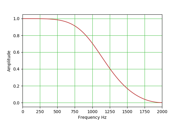
LPF: H(s) = 1 / (s^2 + s/Q + 1)
b0 = (1 - cos(w0))/2
b1 = 1 - cos(w0)
b2 = (1 - cos(w0))/2
a0 = 1 + alpha
a1 = -2*cos(w0)
a2 = 1 - alpha
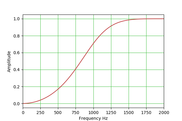
HPF: H(s) = s^2 / (s^2 + s/Q + 1)
b0 = (1 + cos(w0))/2
b1 = -(1 + cos(w0))
b2 = (1 + cos(w0))/2
a0 = 1 + alpha
a1 = -2*cos(w0)
a2 = 1 - alpha
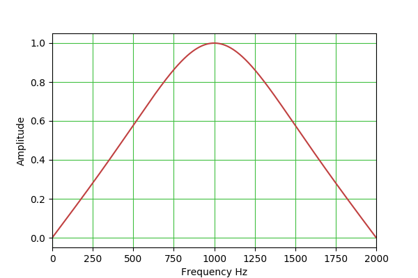
BPF: H(s) = s / (s^2 + s/Q + 1) (constant skirt gain, peak gain = Q)
b0 = sin(w0)/2 = Q*alpha
b1 = 0
b2 = -sin(w0)/2 = -Q*alpha
a0 = 1 + alpha
a1 = -2*cos(w0)
a2 = 1 - alpha
BPF: H(s) = (s/Q) / (s^2 + s/Q + 1) (constant 0 dB peak gain)
b0 = alpha
b1 = 0
b2 = -alpha
a0 = 1 + alpha
a1 = -2*cos(w0)
a2 = 1 - alpha
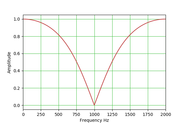
notch: H(s) = (s^2 + 1) / (s^2 + s/Q + 1)
b0 = 1
b1 = -2*cos(w0)
b2 = 1
a0 = 1 + alpha
a1 = -2*cos(w0)
a2 = 1 - alpha
APF: H(s) = (s^2 - s/Q + 1) / (s^2 + s/Q + 1)
b0 = 1 - alpha
b1 = -2*cos(w0)
b2 = 1 + alpha
a0 = 1 + alpha
a1 = -2*cos(w0)
a2 = 1 - alpha
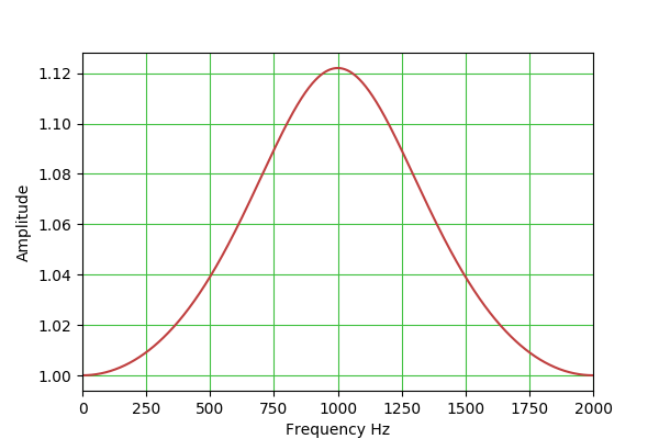
peakingEQ: H(s) = (s^2 + s*(A/Q) + 1) / (s^2 + s/(A*Q) + 1)
b0 = 1 + alpha*A
b1 = -2*cos(w0)
b2 = 1 - alpha*A
a0 = 1 + alpha/A
a1 = -2*cos(w0)
a2 = 1 - alpha/A
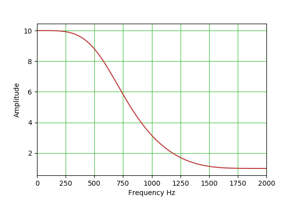
lowShelf: H(s) = A * (s^2 + (sqrt(A)/Q)*s + A)/(A*s^2 + (sqrt(A)/Q)*s + 1)
b0 = A*( (A+1) - (A-1)*cos(w0) + 2*sqrt(A)*alpha )
b1 = 2*A*( (A-1) - (A+1)*cos(w0) )
b2 = A*( (A+1) - (A-1)*cos(w0) - 2*sqrt(A)*alpha )
a0 = (A+1) + (A-1)*cos(w0) + 2*sqrt(A)*alpha
a1 = -2*( (A-1) + (A+1)*cos(w0) )
a2 = (A+1) + (A-1)*cos(w0) - 2*sqrt(A)*alpha
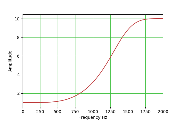
highShelf: H(s) = A * (A*s^2 + (sqrt(A)/Q)*s + 1)/(s^2 + (sqrt(A)/Q)*s + A)
b0 = A*( (A+1) + (A-1)*cos(w0) + 2*sqrt(A)*alpha )
b1 = -2*A*( (A-1) + (A+1)*cos(w0) )
b2 = A*( (A+1) + (A-1)*cos(w0) - 2*sqrt(A)*alpha )
a0 = (A+1) - (A-1)*cos(w0) + 2*sqrt(A)*alpha
a1 = 2*( (A-1) - (A+1)*cos(w0) )
a2 = (A+1) - (A-1)*cos(w0) - 2*sqrt(A)*alpha
FYI: The bilinear transform (with compensation for frequency warping)
substitutes:
1 1 - z^-1
(normalized) s <-- ----------- * ----------
tan(w0/2) 1 + z^-1
and makes use of these trig identities:
sin(w0) 1 - cos(w0)
tan(w0/2) = ------------- (tan(w0/2))^2 = -------------
1 + cos(w0) 1 + cos(w0)
resulting in these substitutions:
1 + cos(w0) 1 + 2*z^-1 + z^-2
1 <-- ------------- * -------------------
1 + cos(w0) 1 + 2*z^-1 + z^-2
1 + cos(w0) 1 - z^-1
s <-- ------------- * ----------
sin(w0) 1 + z^-1
1 + cos(w0) 1 - z^-2
= ------------- * -------------------
sin(w0) 1 + 2*z^-1 + z^-2
1 + cos(w0) 1 - 2*z^-1 + z^-2
s^2 <-- ------------- * -------------------
1 - cos(w0) 1 + 2*z^-1 + z^-2
The factor:
1 + cos(w0)
-------------------
1 + 2*z^-1 + z^-2
is common to all terms in both numerator and denominator, can be factored
out, and thus be left out in the substitutions above resulting in:
1 + 2*z^-1 + z^-2
1 <-- -------------------
1 + cos(w0)
1 - z^-2
s <-- -------------------
sin(w0)
1 - 2*z^-1 + z^-2
s^2 <-- -------------------
1 - cos(w0)
In addition, all terms, numerator and denominator, can be multiplied by a
common (sin(w0))^2 factor, finally resulting in these substitutions:
1 <-- (1 + 2*z^-1 + z^-2) * (1 - cos(w0))
s <-- (1 - z^-2) * sin(w0)
s^2 <-- (1 - 2*z^-1 + z^-2) * (1 + cos(w0))
1 + s^2 <-- 2 * (1 - 2*cos(w0)*z^-1 + z^-2)
The biquad coefficient formulae above come out after a little
simplification.
Biquadratic difference equation flow graph
(horizontal = time, vertical = data flow):

// perform one filtering step
double filter(double x) {
    y = b0 * x + b1 * x1 + b2 * x2 - a1 * y1 - a2 * y2;
    x2 = x1;
    x1 = x;
    y2 = y1;
    y1 = y;
    return (y);
}
This table outlines the properties of the available filter types:
Filter Type Q adj Gain adj Comments Image Bandpass Y N The most generally useful filter type. Low-pass Y N For low-pass and high-pass biquadratic filters, one normally sets Q = 0.707 ($frac{1}{sqrt{2}}$) to achieve a Butterworth filter transfer function with a 3 DB drop at the specified operating frequency. Higher Q settings produce an often-undesirable peak near the center frequency and dynamic instability in operation. High-pass Y N Peak Y Y This filter is a bit tricky to set up, because both Q and gain are effective. The idea is that one can use the gain control to set a nonzero base gain level that applies to all frequencies, then use the frequency and Q controls to set a narrow peak to exceed that level. Note also that, with a negative gain setting, the relation between the plateau and peak is reversed. Notch Y N This filter is more or less the opposite of the "Peak" filter — it creates a narrow rejection band, the width of which is set by the Q control. (But no plateau as with "Peak".) Lowshelf N Y Lowshelf and highshelf filters provide a sort of "plateau" effect, under control of the gain setting, and not unlike the "Peak" filter described above. Note that negative gain settings reverse the identity of the filter — lowshelf becomes highshelf and the reverse. Highshelf N Y