很久没来写博客了,感觉自己也懈怠了很多,最近毕业,工作,身份变化很大,烦心事也很多,对自己的第一份工作不是特别满意,所以决定自学一下机器学习,给自己留一条后路。希望多日以后的自己再看到这篇文章的时候还能记起当时痛苦的心情。
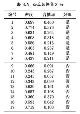
题目是:编程实现对率回归,并给出西瓜数据集3.0α上的结果。
西瓜数据集如下:
在这里我们主要使用了sklean,matplotlib,numpy和pandas几个库,由于sklearn中自带了有关线性回归的算法,所以可以直接调用,另外使用了matplotlib对其进行可视化处理。
代码如下:
 1 import numpy as np
 2 import matplotlib.pyplot as plt
 3 import pandas as pd
 4
 5 from sklearn import model_selection
 6 from sklearn.linear_model import LogisticRegression
 7 from sklearn import metrics
 8
 9 # load the CSV file as a numpy matrix
10 dataset = pd.read_csv('F:PythonTestMachine Learningwatermelon3a.csv')
11
12 # separate the data from the target attributes
13 X = dataset[['密度','含糖率']]
14 y = dataset['好瓜']
15 good_melon = dataset[dataset['好瓜']==1]
16 bad_melon = dataset[dataset['好瓜']==0]
17
18 # draw scatter diagram to show the raw data
19 f1 = plt.figure(1)
20 plt.title('watermelon_3a')
21 plt.xlabel('density')
22 plt.ylabel('ratio_sugar')
23 plt.xlim(0,1)
24 plt.ylim(0,1)
25 plt.scatter(bad_melon['密度'], bad_melon['含糖率'], marker = 'o', color = 'k', s=100, label = 'bad')
26 plt.scatter(good_melon['密度'], good_melon['含糖率'], marker = 'o', color = 'g', s=100, label = 'good')
27 plt.legend(loc = 'upper right')
28
29
30 # generalization of test and train set
31 X_train, X_test, y_train, y_test = model_selection.train_test_split(X, y, test_size=0.5, random_state=0)
32
33 # model training
34 log_model = LogisticRegression()
35 log_model.fit(X_train, y_train)
36
37 # model testing
38 y_pred = log_model.predict(X_test)
39
40 # summarize the accuracy of fitting
41 print(metrics.confusion_matrix(y_test, y_pred))
42 print(metrics.classification_report(y_test, y_pred))
43 print(log_model.coef_)
44
45 theta1,theta2 = log_model.coef_[0][0],log_model.coef_[0][1]
46 x_pred = np.linspace(0,1,100)
47 line_pred = theta1+theta2*x_pred
48 plt.plot(x_pred,line_pred)
49
50 plt.show()
代码比较简单,好久没用python了,对其中的一些库和相应的操作有些不熟悉了,所以还是花费了很长的时间。主要是这些库的操作不是很熟练,包括使用matplotlib进行画图,使用了linspace这个函数,然后还有通过调用pandas的read_csv进行数据集的提取,以及使用sklearn调用线性回归等。有关线性回归的几个点摘抄如下,来自https://blog.csdn.net/qq_29083329/article/details/48653391
参数:
fit_intercept: 布尔型,默认为true
说明:是否对训练数据进行中心化。如果该变量为false,则表明输入的数据已经进行了中心化,在下面的过程里不进行中心化处理;否则,对输入的训练数据进行中心化处理
normalize布尔型,默认为false
说明:是否对数据进行标准化处理
copy_X 布尔型,默认为true
说明:是否对X复制,如果选择false,则直接对原数据进行覆盖。(即经过中心化,标准化后,是否把新数据覆盖到原数据上)
n_jobs 整型, 默认为1
说明:计算时设置的任务个数(number of jobs)。如果选择-1则代表使用所有的CPU。这一参数的对于目标个数>1(n_targets>1)且足够大规模的问题有加速作用。
返回值:
coef_ 数组型变量, 形状为(n_features,)或(n_targets, n_features)
说明:对于线性回归问题计算得到的feature的系数。如果输入的是多目标问题,则返回一个二维数组(n_targets, n_features);如果是单目标问题,返回一个一维数组 (n_features,)。
intercept_ 数组型变量
说明:线性模型中的独立项。
注:该算法仅仅是scipy.linalg.lstsq经过封装后的估计器。
方法:
predict(X) 使用训练得到的估计器对输入为X的集合进行预测(X可以是测试集,也可以是需要预测的数据)。
score(X, y[,]sample_weight) 返回对于以X为samples,以y为target的预测效果评分。
set_params(**params) 设置估计器的参数