proof-theoretic
ways to derive facts
-
bottom up: starting from the known facts and deriving all possible new facts
technique: fixpoint
-
top-down: starting from a fact to be proven and attempts to demonstrate it by deriving lemmas that are needed for the proof
technique: SLD
syntax of datalog
-
datalog程序是由有限条规则(rule)组成,出现在rule head中的变量在rule body中应全部包含
-
datalog 程序中的常量(constant)用 adom(P) 表示,datalog规则实例(instance)中出现的常量用 adom(I) 表示,用 adom(P,I) 来表示 (adom(P)cup adom(I))
-
edb(P) : extensional database(input data) schema extensional relation occurring only in the rule body
idb(P) : intensional database(program) schema intensional relation occurring only in the rule head
sch(P) : union of edb(P) and idb(P); -
semantics of P: maps instances over edb(P) to instances over idb(P)
datalog & logic programming
- predicate in logic-based languages ( ightarrow) relation name in datalog
- logic programming permits function symbols,but datalog does not
- datalog program P is viewed as defining a mapping from instances over the edb to instances over the idb,while in logic program, the base data is incorporated directly into the program, so if the base data changes, the logic program itself is changed
Model-Theoretic Semantics
-
A datalog program can be viewed as a set of (particular) Horn clauses(disjunction of literals of which at most one is postive):
a datalog rule[ ho : R_1(u_1) leftarrow R_2(u_2), ldots ,R_n(u_n) ]the related logical sentence
[forall x_1, ldots ,x_m(R_1(u_1)) leftarrow R_2(u_2) land ldots land R_n(u_n)) ]equivalent to
[forall x_1, ldots ,x_m(R_1(u_1)) lor lnot R_2(u_2) lor ldots lor lnot R_n(u_n)) ] -
smallest model: the semantics of P on input I, denoted P(I), is the minimum model of P containing I
- $ P = { r_1,ldots,r_n}, sum P = r_1 land ldots land r_n $
- the answer is a particular model of (sum p)
- I over sch(P) is a model of (sum p) (I satisfies (sum p)) if $ I vDash r_1 land ldots land r_n $
define (B(P,I)) : the instance over sch(P) ,is a model of P containing I, and P(I) is a subset of it
- For each R in edb(P), a fact R(u) is in B(P,I) iff it is in I; and
- For each R in idb(P), each fact R(u) with constants in adom(P,I) is in B(P,I).
Fixpoint Semantics
an implementation of the model-theoretic semantics
- the immediate consequence operator: produces new facts starting from known facts; P(I) can also be defined as the smallest solution of a fixpoint equation involving this operator
- For each instance K over sch(P), (T_p(K)) consists of all facts A that are immediate consequences for K and P.
- T is monotone if for each I, J, I ⊆ J implies T (I) ⊆ T (J).
- K is a fixpoint of T if T (K) = K.
- (P(I)) is a fixpoint of (T_p), and it is the minimum fixpoint containing I.
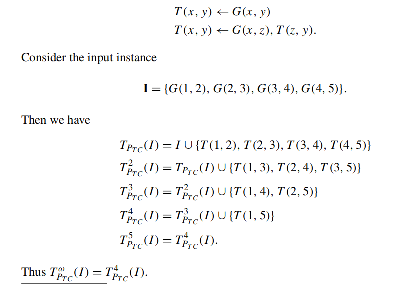
- Let N be the number of facts in B(P,I), the sequence ({T_P^i(I)}_i) reaches a fixpoint after at most N steps, and this fixpoint is denoted by (T_p^w(I))
- (stage(P,I)): The smallest integer i such that (T_P^i(I) = T_P^w(I)), and P(I) = stage(P,I) ≤ N = |B(P,I)|
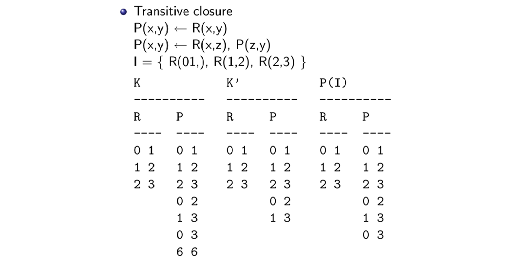
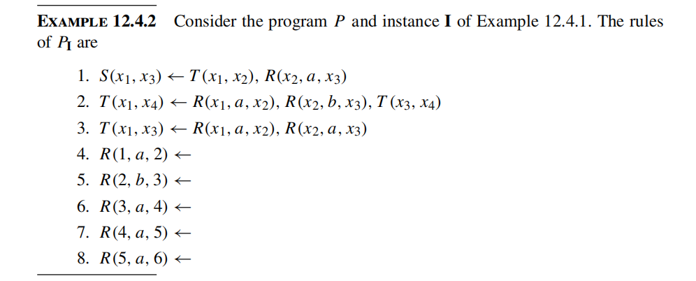
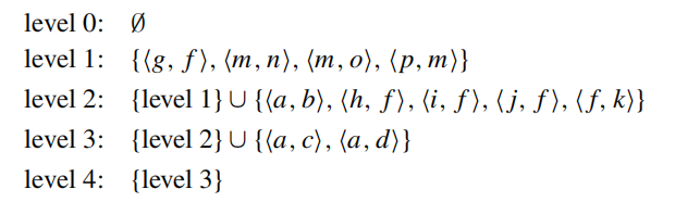
example
B(P,I) 的确定:
- 在(P_{TC})中,G为edb关系谓词,T为idb关系谓词,根据define1.1,I中所有G规则对应的实例事实都在B(P,I)中,所以B(P,I)={G(1,2),G(2,3),G(3,4),G(4,5)}
- 该例中adom(P,I)={1,2,3,4,5},而I中没有包含adom中元素的T事实,所以没有加入到B(P,I)的事实,因此最后|B(P,I)|=4
Evaluation
- (section4.5) for each nr-datalog program P, there exists a constant d such that for each I over edb(P), stage(P,I) ≤ d(e.i. the fixpoint is reached after a bounded number of steps)
Proof-Theoretic Approach
-
Proof trees
provide proofs of facts. It is straightforward to show that a fact A is in P(I) iff there exists a proof tree for A from I and P- bottom-up: fixpoint
- top-down: SLD resolution
-
SLD resolution
warm up
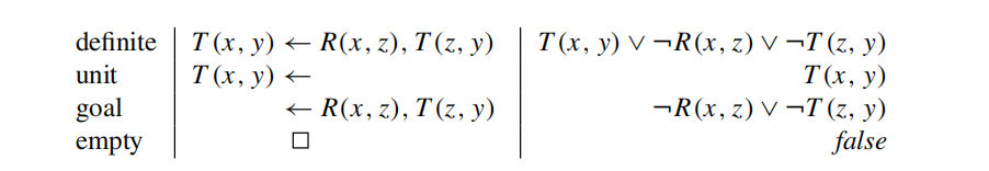
A ground clause is a clause with no occurrence of variables
the datalog program (P_I) consisting of the rules of P and { one rule R(u) ← }for each fact R(u) in I, so a datalog unit clause will be ground.
-
each intermediate step of the top-down approach consists of obtaining a new goal from a previous goal. Finally, the procedure is deemed successful if the final goal reached is empty.
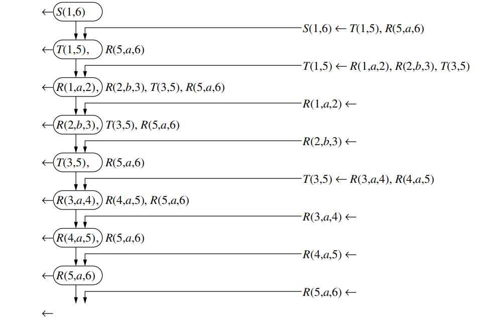
-
refutations proofs: try to refute the negation of the goal which can be denoted as a query([i.e., ¬S(1, 6) or ← S(1, 6))
more general case
- variable renaming
- most general unify
evaluation
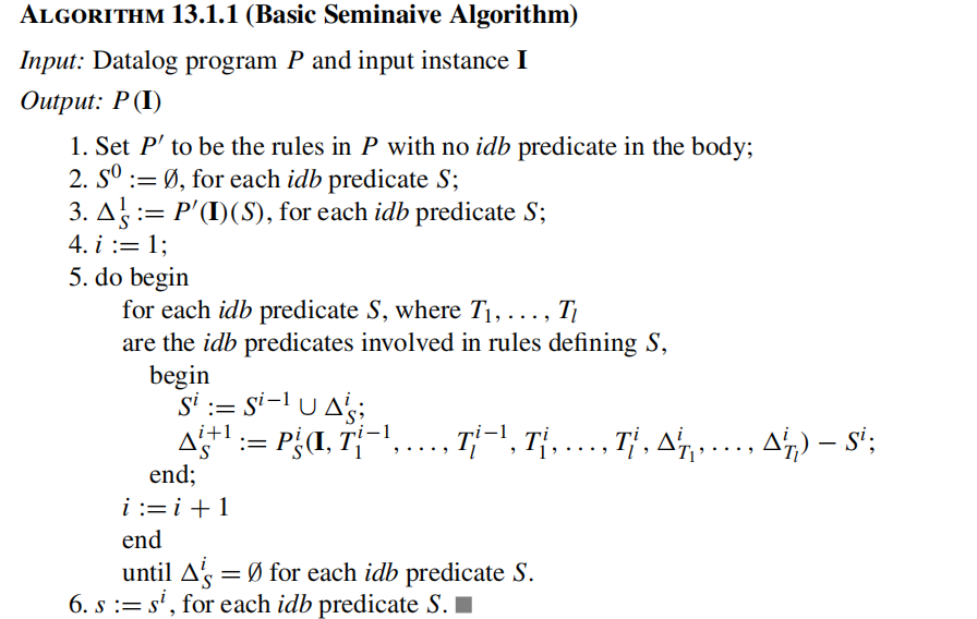
semi-naive bottom-up evaluation
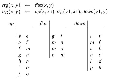
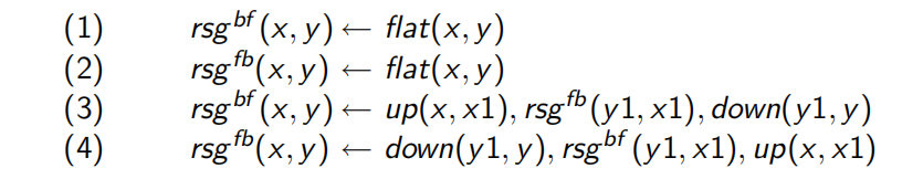
RSG program and input instance (I_0)
apply bottom-up algorithm(naive) until a fixpoint has been reached
Analysis: a amount of redundant computation is done, because each layer recomputes all elements of the previous layer. This is a consequence of the monotonicity of the TP operator for datalog programs P.
Semi-naive algorithm: focus on the new facts generated at each level RSG'
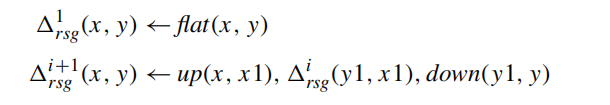
- (Delta_{rsg}^i): containing facts in rsg newly inferred at the ith stage of the naive evaluation
- (delta_{rsg}^i): the value of (Delta_{rsg}^i) when (T_{RSG}^′) reaches a fixpoint on I
- for each (i ge 0): (rsg^{i+1} - rsg^i subseteq delta_{rsg}^{i+1} subseteq rsg^{i+1}), therefore (RSG(I)(rsg) = cup_{1 le i}(delta_{rsg}^{i+1}))
improvement 1: using (rsg^i − rsg^{i−1}) in place of (Delta_{rsg}^i) in the body of the second “rule” of RSG′.
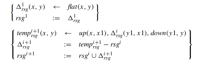
improvement 2: it's useful when a given idb predicate occurs twice in the same rule

so, replace the two rules for (temp^{i+1}) to further reduce redundancy

more general case
Consider a rule in P where R is edb predicates and T is idb predicates:
Construct for each (jin[1,m]) and (i ge 1) the rule:
Let (P_s^i) represent the set of all i-level rules, suppose now that (T_1,ldots,T_l) is a listing of the idb predicates of P that occur in the body of a rule defining S, then
to denote the set of tuples that result from applying the rules in (P_S^i) to given values for input instance I and for the (T_j^{i-1},T_j^i,and Delta_{T_j}^i)
we now have the following:
top-down : QSQ
A primary motivation for the top-down approaches to datalog query evaluation is to avoid, to the extent possible, the production of tuples that are not needed to derive any answer tuples, but focus attention on relevant facts.
The starting point for these algorithms (namely, the query to be answered) often includes constants; these have the effect of restricting the search for derivation trees and thus the set of facts produced.
the query-subquery(QSQ) framework:
- focus on relevant data
- avoid deriving unnecessary tuples

adornment and adorned rules
a top-down evaluation of a query in which constants occur can be broken into a family of “subqueries” having the form ((R^γ,J)), where γ is an adornment for idb predicate R, and J is a set of tuples that give values for the columns bound by γ .Expressions of the form ((R^γ,J)) are called subqueries
left-to-right evaluation to detemine the adornment:
- All occurrences of each bound variable in the rule head are bound
- all occurrences of constants are bound, and
- if a variable x occurs in the rule body, then all occurrences of x in subsequent literals are bound.
supplementary relations and QSQ templates
provides data structures that will remember all of the values needed during a left-to-right evaluation of a subquery. the body of a rule may be viewed as a process that takes as input tuples over the bound attributes of the head and produces as output tuples over the variables (bound and free) of the head.
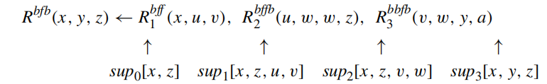
the supplementary relation is determined as follows
- For the 0th (i.e., zeroth) supplementary relation, the attribute set is the set X0 of bound variables of the rule head; and for the last supplementary relation, the attribute set is the set Xn of variables in the rule head.
- For i ∈ [1, n − 1], the attribute set of the ith supplementary relation is the set Xi of variables that occur both “before” Xi (i.e., occur in X0, A1,...,Ai) and “after” Xi(i.e., occur in Ai+1,...,An, Xn).
The QSQ template for an adorned rule is the sequence (sup0,...,supn) of relation schemas for the supplementary relations of the rule
the kernel of the technique
-
input: program + query
-
construct an adorned rule for each adornment of each idb predicate in P and for the query q
-
construct QSQ template for each adorned rule i and the supplementary relation variables (sup_j^i) construct also : for each idb R and adornment γ
- the variable (ans_R^γ) of arity arity(R)
- the variable (input_R^γ) of arity bound(R, γ)
-
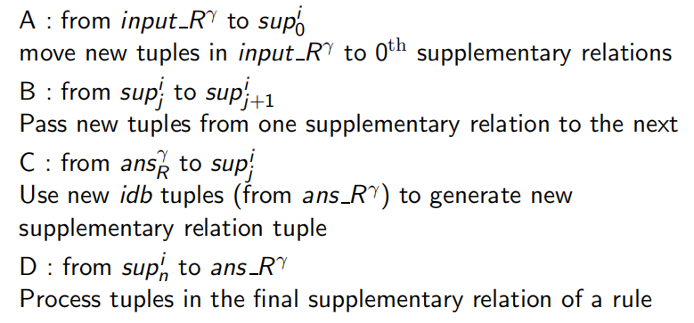
setup the QSQ algorithm:
- initialize: use the query to give initialize values to input_(R^{gamma})
- four kinds of steps in the execution(details in 321~322):
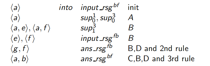
example
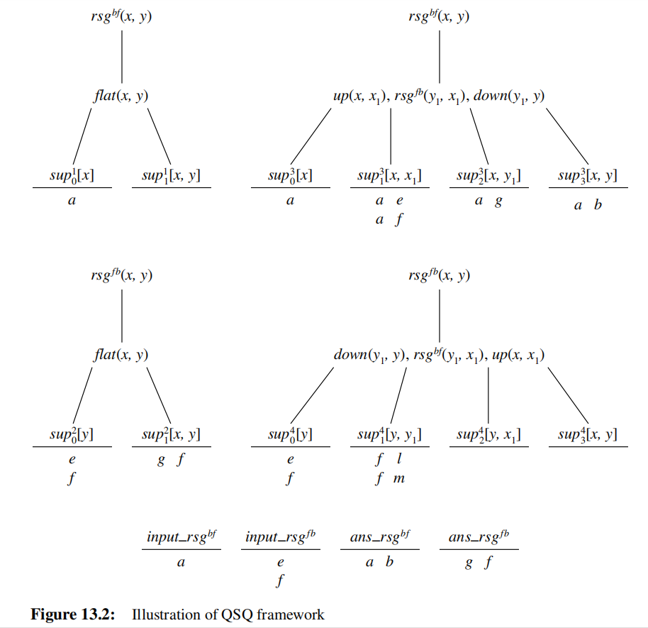
analysis